- Squared Correlation: R2 or RSquare
We have just used the squared correlation, R2 = corr(x,y)2, to select the best set of transformations for x and y. We translate the fundamental properties from raw to squared correlations:- R2=1 <=> corr(x,y)=+1 or -1 <=> x, y are in perfect linear association (ascending OR descending)
- R2= 0 <=> x and y are in no linear association whatsoever.
- R2 is unit-free.
In Module 3 there will be an interpretation of R2 as "fraction of variance explained". For now we are content with the interpretation of R2 as a measure of
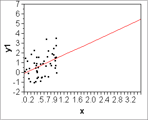
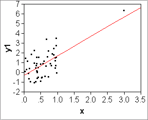
diagonal elongation of the data cloud in the x-y plain. The more elongated the best-fitting ellipse, the higher R2.
Recall how to find "density ellipses" in JMP:
JMP: Analyze > Fit Y by X > pick X, Y; OK > red diamond > Density Ellipse > 0.95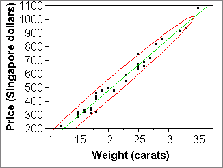
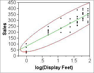
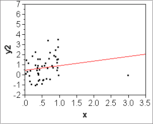
R2=0.978 R2=0.815 - Root Mean Square Error or RMSE: [slides 2-9, 2-10]
RMSE: measure of quality of a fit, on the scale of the response.
- Formula: RMSE = (RSS/(n-2))1/2
- The RMSE describes how well our predictions fit the observations.
- More precisely, it estimates the SD of errors around the true line.
- If the data are nice, that is, the errors around the true line
are normally distributed, then:
- the true line +- RMSE contains 68% of the data;
- the true line +- 2*RMSE contains 95% of the data.
- Compare:
- The RMSE measures the quality of fit by the vertical width of a band that contains 68% of the data.
- R2 measures the quality of fit in terms of diagonal elongation of the x-y points;
- RMSE is not symmetric in x and y;
- R2 is symmetric in x and y.
- JMP: 3rd number under "Summary of Fit", called "Root Mean Square Error".
- RMSE and log(y) fits: Example Used Car data
In JMP, the log(y)-model shows RMSE=0.114923, which may seem useless, because we don't do predictions on the log(y) scale. But JMP also shows an RMSE under "Fit Measured on Original Scale", 0.718, which describes the spread of the data around the fitted curve. It says our predictions have a 68% uncertainty of about +-$720, and 95% uncertainty of about +-$1,440. Then again, this might seem not right because as the values decrease, their variability should decrease proportionately. So maybe the RMSE on the log(y)-scale is the right one to use.
- Faking data:
- Q: What could prices of other Diamond Ring data have looked like?
- -> Simulate alternative data in JMP!
- Q: How?
- We know how to compute predictions from linear equations, but these predictions don't look like real response values. Unlike real data, they don't have variability off the straight line.
- A: Use a straight-line formula and add variability.
- Example: The Simulated Diamond Ring data have an additional column, "Price (simulated)", which implements the idea. If you look at its formula (R-click column label > Formula), you will see something like this:
Price = -260 + 3720*Weight + 32*RandomNormal() - Thought experiment: Let us assume that we know the true intercept, slope, and RMSE.
- Assume the true intercept and slope values are -260 and 3720.
- Assume also the variability around the straight line is normal, has true mean m=0 and true SD s=32.
- (We gleaned these values from the JMP analysis, which gave an estimated intercept -259.6, slope 3721, and RMSE=31.84.)
- Seeing Sample-to-Sample Variability in JMP:
- JMP: R-click "Price (simulated)" > Formula > Apply
With every click on "Apply", the column gets filled with another set of numbers that look very similar to the actually observed data.
How convincing are these fake response values? Check graphically.- Look at the data generated by the formula with scatterplots:
- First make a scatterplot of the real data:
- X="Weight (carats)"; "Price (Singapore Dollars)"
- Then make three or so scatterplots of simulated data:
- X="Weight (carats)"; "Price (simulated)",
- clicking "Apply" in the formula window between each plot.
- An example is shown in the
plots below.
- Think of the observed data as generated by this formula!
- The formula gives us a means to simulate sample-to-sample variation, assuming that it is a good "model" for the real data.
We think of the formula as a model for the data! [Slide 2-2 uses the term "data generating process".] 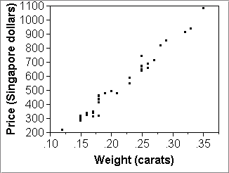

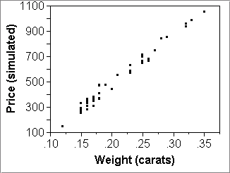

The above pictures give the impression that the three simulated datasets are pretty good fakes of the real thing (top left picture). The model seems to work quite nicely as a summary of the data.
(There are some small discrepancies between the actual and the simulated data. The actual data seem to have a little less variability than their simulated cousins. After perusing the actual prices, one sees that there is a slight preponderance of round values, such as multiples of $10 and $5. A good data forger would round the simulated prices first to whole dollars and then some with small probability to nearest multiples of 10 or 5. Reduction of variability due to rounding is typical for monetary variables.)
- Model for the population:
yi = b0 + b1 *xi + ei where ei are i.i.d. N(0,s2)response = signal + noise (general) = straight line + normal variability (special)As always, Greek letters stand for true but unknown population numbers. They are to be estimated by their sample-analogs b0 and b1, written in Roman letters. -
Essential: The straight line wants to capture
the true means of y given any x value,
e.g., true mean price for weights 0.12, 0.15, ...carats.
This is expressed by errors with true mean zero for any fixed xi: m(xi) = 0. Another way of writing the model is as follows:y | x ~ N(b0+b1*x, s2) Meaning: The distribution of y at x is normal with true mean m(x)=b0+b1*x and true constant SD s. -
Q: Who says these true means sit on a straight line?
A: Nobody. We're assuming it.
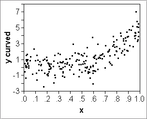
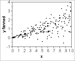
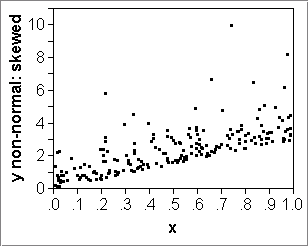
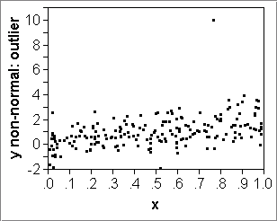
Diagnostic: A scatterplot can show whether this is a reasonable assumption (counter-example: display.JMP). -
Q: Who says the errors are i.i.d. normal with a true SD=sigma?
A: Nobody. We're assuming it.
Diagnostic: We'll get to that shortly. - Models and Estimation: [slides 2-6...2-8]
- With Least Squares we estimate
- the true parameter values b0, b1, s
- with estimated values b0, b1, s.
- We also estimate
- the true means m(xi) = b0 + b1 * xi
- with estimated means yhati = b0 + b1 * xi
- -> FITS yhati (also: "fitted values", "predicted values")
- and true errors ei= yi - m(xi)
- with estimated errors ei = yi - yhati
- -> RESIDUALS ei
- with estimated means yhati = b0 + b1 * xi
- Setup:
- The assumption is that there exists a true straight line that contains the true mean of y for each value of x.
- Least Squares gives us an estimated straight line that contains an estimated mean of y for each value of x.
- The true straight line is fixed.
The estimated straight line has sample-to-sample variation.
- Illustration of regression with
i,
but we hope that
1) the xi's in hand describe the important factors and
2) the unknown factors are many and small and additive,
so the central limit theorem justifies lumping them
into "errors", "noise", "unexplained variability"
that looks roughly normally distributed.
Example: We hope weight in carats is the primary factor driving prices,
and other factors (purity, brightness, shape,...) are minor.
If we had data for these other factors, we could use statistical tests
to see whether these factors are minor or not
- THE WEIRDNESS OF THE REGRESSION MODEL: Sample-to-sample variability in y but not x. Note for the diamond ring data we only modeled the variability of prices yi given the same weight values xi. We did NOT model the variability of weights xi, although we could have done so in principle. But this is NOT done in regression: REGRESSION IS "CONDITIONAL ON THE x-VALUES". Regression only models sample-to-sample variability in y but keeps the x-values fixed. In the diamond data, the regression model assumes samples with the same weights but (slightly) varying prices. (Compare the simulation in utopia.JMP: There, one generates variability in the x's also, namely, with a uniform distribution, but this is not part of the regression model. Variability in the x's would often be more realistic.)
- SIMULATION FOR MODEL DIAGNOSTICS: Although we interpreted the above simulation of the diamond data as a thought-experiment, we can obviously use it as a diagnostic: Use estimates of slope, intercept, SD as if they were the true values, then simulate data from the resulting formula, and check whether the simulated and observed data look similar.
(This approach is called "predictive model check" and unfortunately not widely known. It is also related to something called "parametric bootstrap".) - THE WEIRDNESS OF THE REGRESSION MODEL: Sample-to-sample variability in y but not x. Note for the diamond ring data we only modeled the variability of prices yi given the same weight values xi. We did NOT model the variability of weights xi, although we could have done so in principle. But this is NOT done in regression: REGRESSION IS "CONDITIONAL ON THE x-VALUES". Regression only models sample-to-sample variability in y but keeps the x-values fixed. In the diamond data, the regression model assumes samples with the same weights but (slightly) varying prices. (Compare the simulation in utopia.JMP: There, one generates variability in the x's also, namely, with a uniform distribution, but this is not part of the regression model. Variability in the x's would often be more realistic.)