- Q: Does x matter to predict or explain y?
- Diamond ring prices: No question, weight is the major factor that drives prices.
- Wine displays: Sure, feet of display space seems to have a large influence on sales.
- Used cars: Of course, age is the driving factor of price.
(Testing becomes a lot more important in multiple regression with more than one predictor variable. It will help us weed out unimportant variables.) - Q: How precise are our estimates?
A: Confidence intervals (CIs)
=> We want CIs for b1, b0, and mean response values.
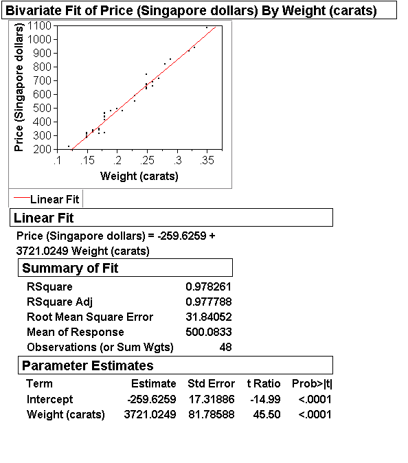
Example: Diamond ring prices.
We will see that the average price $3,720 of an additional carat will have the 95% CI = (3720-160, 3720+160) = (3560, 3880). More realistically, the CI for an additional 1/10 carat is (356, 388).This seems like a useful thing to know, for example, during sales negotiations: If a buyer proposes 1) to buy a larger ring with 2/10 more carat instead of a smaller one, and 2) to pay 400 more and throw in an heirloom ring of his that we estimate to be worth 220, do we go for the deal? Maybe not: Our CI for an additional 2/10 carats is (712, 776), so 400+220=620 falls short of the range where we think the average price of an additional 2/10 carats should be.
(We'll get to know other ways of answering such questions with prediction intervals that might be more satisfactory.) - Q: In what range should we expect future observations to fall?
A: Prediction intervals (PIs)
Example: In what range should we expect prices to fall for 0.4 carat diamonds? We will see that (1156, 1301) is a reasonable guess for a 95% prediction interval.
- We approach things from a practical point of view and give
underpinnings later. We argue by analogy to inference for means:
like means, slopes and intercepts have standard errors, CIs, and
statistical tests, and they work very much the same way. We
elaborate for the slope, the parameter of main interest:
- Standard error, SE(slope)
- Confidence intervals, CI(slope): CI = (b1 - 2*SE, b1 + 2*SE)
- t-ratio for the slope: t=b1/SE(slope)
- p-value
We explain these quantities in a minute, but first we show where to find them in JMP.
- Standard error, SE(slope)
- JMP output: We use (as usual) the Diamond Ring data.
We are familiar with the linear equation with intercept and
slope, as well as R2 and RMSE. The estimated intercept b0 and slope b1
can be found a second time in a section with title "Parameter Estimates".
In this section we also find a column with SEs ("Std Error"),
a column with t-statistics ("t Ratio"), and a column with p-values ("Prob>|t|").
(Ignore other sections such as "Lack of Fit" and "Analysis of Variance" for now.)
- We elaborate on the meaning and use of these quantities:
- The SE(slope) is the standard deviation of the estimates b1
under sample-to-sample (dataset-to-dataset) variability.
Standard errors measure the uncertainty of estimates
due to sample-to-sample variability.
- The CI(slope) is a random interval that will catch the
true slope b1 95% of times; in other words:
the true b1 is in CI(slope) for 95% of samples (=datasets).
- Before interpreting t-ratios and p-values, we must understand
that the conventional null hypothesis H0 is: b1=0.
Why? Because if the true slope is b1=0, then the predictor x is irrelevant for predicting or explaining the response y (diamond weight would be irrelevant for price, which it isn't).
As we said earlier, this conventional null hypothesis is mostly not very meaningful right now because with a single predictor even weak effects tend to be significant even for small sample sizes. - We reject H0: b1=0 at the 5% significance level
if any and all of the following equivalent conditions are satisfied:
- |b1| > 2*SE, that is, either b1 > 2*SE or b1 < -2*SE
- 0 is not in the 95% CI
- |t|>2, that is, either t>2 or t<-2
- p-value < 0.05
These conditions all describe the situation that the observed estimate b1 and the assumed parameter value b1=0 are too far apart to be compatible: b1 is too unlikely to be observed under the assumption b1=0. The yard stick for measuring distance between b1 and anything else is the SE, because the SE measures the uncertainty in b1.
The most confusing among the above conditions for rejection of H0 is in terms of the p-value. Recall: the p-value is a measure of evidence in favor of H0 on a probability scale. In order to reject H0, we want this evidence for H0 to be small, namely, less than 0.05 (a convention corresponding to 0.95 confidence for CIs).
Slides 3-3 and 3-5 show how to test any other slope value also, such as b1=$3,800 for the diamond data. We just check whether b1=3721 and b1=3800 are further apart than two SEs (=82). They are not: |3721-3800|=79 < 2*82=164. Hence an assumed price of 3800 per additional carat could not be rejected based on the data.
- Why is the intercept rarely tested? It's not often of interest. Testing the intercept can be of interest if y=cost/price and x=quantity, in which case intercept=fixed cost. One might ask: Is there fixed cost at all? This suggests testing the null hypothesis that true fixed cost is zero, b0=0. We will reject if b0> 2*SE(intercept).
- The SE(slope) is the standard deviation of the estimates b1
under sample-to-sample (dataset-to-dataset) variability.
Standard errors measure the uncertainty of estimates
due to sample-to-sample variability.
- Analysis of the standard error of slopes:
Preliminary remark: From now on se = RMSE is our new notation for the estimate of s, the spread of the response values around the true line:
- se = RMSE = [ ( e12+...+en2 )/(n-2)]1/2
- There exists an explicit formula for the SE of the slope, shown on
slide 3-2:
                       se    1
             SE(b1) = --- * --
                       n1/2  sX
We will never use the above formula for actual calculation of SE(b1) since JMP does that. But we find the formula insightful.First a reminder: sX is the simple standard deviation of the x-values.
- sX = [ (x1-x)2+...+(xn-x)2 ]1/2
a measure of horizontal spread on the x-axis - se = [ e12+...+en2 ]1/2
a measure of vertical spread off the fitted line
- sX = [ (x1-x)2+...+(xn-x)2 ]1/2
- Interpretation of the formula for the standard error of the slope:
- It is good to have a large sample size n:
as n increases, the SE goes to zero like 1/n1/2, just like the SE of the mean in pre-term. Again, we need 4 times as much data to cut the SE by a factor of 2. - It is good to have a small standard deviation se around the line. All other things being equal, SE(slope) is directly proportional to se.
- It is good to have a large spread of the x-values: the SD of the x-values in the denominator shows that, all things being equal, a larger sX entails a smaller SE(b1).
- It is good to have a large sample size n:
- Implications for outlier analysis:
- We don't like vertical outliers: they inflate se.
se is the main quantity affected by vertical outliers.
We hope we can remove them from the data based on subject-matter judgement, such as the coincidence of an inventory sale with a particular mass mailing as in the Direct Mail data used in slides 2-17 and 2-18. - We like horizontal outliers, that is, leverage points: they inflate sX,
which drives down SE(b1).
When we spot a leverage point, we hope it is compatible with the majority of the data in the sense that the slope b1 does not change drastically when the point is removed. We also hope to find arguments that the leverage point is likely to be typical for future data with x-values that are similarly extreme.
- We don't like vertical outliers: they inflate se.
- se = RMSE = [ ( e12+...+en2 )/(n-2)]1/2
- The estimated line yhatx = b0 + b1*x approximates the true regression line
m(x) = b0 + beta1*x. If this is so, we should think that there
ought to exist an SE for yhat(x) and therefore a CI around yhatx that
catches the true m(x) about 95% times (sample-to-sample). Indeed:
                     se        (x-x)2
         SE(yhatx) = --- ( 1 + ----- )1/2
                     n1/2        sX2
where we use the more intuitive abbreviation se = RMSE. The 95% CI is- (yhatx - 2*SE(yhatx), yhatx + 2*SE(yhatx))
Why would we show this arcane formula for SE(yhatx) above?
Not for calculations (JMP does that). Again, it's for a qualitative insight:- SE(yhatx) shrinks at the rate of 1/n1/2.
- SE(yhatx) gets larger as x moves away from x.
SE(y) = sY/n1/2. An implication is that in order to double the precision of y, i.e., to cut SE(y) in half, we need 4 times as much data. The same holds for yhatx.The second point is new: SE(yhatx) = se/n1/2 only for x=x. As x moves away from x, SE(yhatx) grows, that is, the CI widens! The growth is slow, though, as we can convince ourselves in examples.
In summary, x=x is the fulcrum where the estimated lines wobble the least under sample-to-sample variability.Fine print: The above CI holds only if the SRM is correct. If there is undiscovered curvature or heteroscedasticity, the CI for yhatx is not valid, meaning, the coverage of the CI will not be 95%.
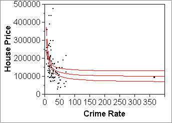
- SE(yhatx) in JMP:
Fit Y by X > pick X and Y > Fit Line or Special > click red diamond "Linear Fit" or "Transformed Fit..." > Confid Curves FitExamples: Used Cars data (left) and the Philadelphia Crime data (right)
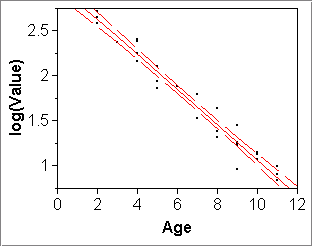
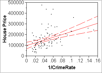
Note the above two plots do linear fits (Fit Line) to transformed variables that obviously have been computed with JMP formulas. If we do the same thing but on the untransformed variables but let "Fit Special" do the transformation, then the CI band is shown on the plot of the original, untransformed variables:
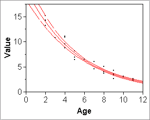
- (yhatx - 2*SE(yhatx), yhatx + 2*SE(yhatx))
-
Recall the distinction between CIs and PIs, confidence intervals and
prediction intervals (from pre-term 603, slide 9-3):
- CIs contain the true parameter 95% of times under sample-to-sample
variability.
- CIs are of the form "estimate +- 2*SE".
- PIs contain 95% of future observations.
In regression this means: 95% of future y's at a given x
(95% of future diamond ring prices for a given fixed weight in carats).- PIs are of the form "estimate +- 2*SD".
- CIs are of the form "estimate +- 2*SE".
- CIs contain the true parameter 95% of times under sample-to-sample
variability.
-
In Deliverables (4) of the Individual Project (Installment 1) you are asked
to do the second: produce two intervals that capture 95% of Total Costs of
future orders, given order sizes of 200 Units and 4000 Units, respectively.
-
We said once that "regression line +- 2*s" contains 95% of the data.
That's correct for the true regression line (m(x)=b0+b1*x)
and the true SD of the errors (s):
- (m(x) - 2*s, m(x) + 2*s)
contains 95% of future observations y at x.
Replacing the truth with estimates (yhat(x) = b0 + b1*x) works ok if we're not extrapolating outside the range of observed x-values:- (yhat(x) - 2*se, yhat(x) + 2*se)
will contain about 95% of future observations y at x.
(Recall se = RMSE.)- If we're extrapolating, we should account for the sample-to-sample variability of yhat(x), which might be sizable at distant x-values for which we have no experience. From the previous section on SE(yhatx), we know that variability of yhatx can be substantial if x is far from x. The formula for the prediction band that adjusts for the sample-to-sample variability of yhatx is as follows: First define the prediction error estimate
- PE(yx) = [ SE(yhatx)2 + se2 ]1/2
Then the 95% prediction interval at x is:- ( yhatx - 2*PE(yx), yhatx + 2*PE(yx) )
See slide 3-9, bottom. We won't use this formula for actual calculations either (JMP will do it). We find the formula interesting, though, because it shows in what way the naive band based on +-2*se gets adjusted for the obvious fact that the more distant x is from x, the less we know about where the responses are going to fall.- JMP, method 1: reading values off the scatterplot with the cross-hair cursor
- Analyze > Fit Y by X > pick X, Y; OK > red diamond: Fit Special... > pick transformations; OK; red diamond next to "Transformed Fit..." > Confid Curves Indiv (This is JMP's unfortunate name for PIs at all x-values, drawn as two curves.)
- Click "+" next to the lense, depress on the plot: cross-hair appears
- Read off the upper and lower 95% PI limits at x=200 and x=4000.
- If necessary, zoom in or out, by changing the min and max of the axes: right-click on axis numbers > Axis Settings > ... change Minimum and Maximum.
- JMP, method 2:
- First create columns with transformed variables, such as logs. This method works directly only on the scale on which a straight line is fitted.
- Add two rows: Rows (at top) > Add rows... > 2
- Fill in the values 200 and 4000 in the new rows of the Units column.
- Analyze > Fit Model > pick Y; click x-variable, click "Add"; "Run Model" > red diamond: Save Columns > Indiv Confidence Interval (again JMP's unfortunate name for PI)
- Two new columns will have appeared in the spreadsheet, containing upper and lower PI bounds for all rows in the spreadsheet, including the two additional rows.
- Back-transform if you used a y-transform. To this end form two new columns with the formula "Exp(...)", if you used a log(y) transform.
- (m(x) - 2*s, m(x) + 2*s)
- We often hear R2 described as "proportion of total
variation explained by the regression" or, more sloppily,
"fraction of explained variance". What is this based on?
Part of learning a new field is also learning about its conventions. - Q: If R2 is a fraction, what is the the denominator?
A: sY2 = [(y1-y)2+...+(yn-y)2]/(n-1),
which describes the total variation of the y-values ignoring the x-values.
To reconstruct the interpretation of R2 as "fraction of variation explained by the regression", we interpret- se2 as the "variance unexplained by the regression". But if
- sY2 is "total variance", then
- sY2-se2 is the "variation explained by the regression", hence
- [ sY2-se2 ]/sY2 is the "fraction of variation explained by the regression".
- se2 = (e12+...+en2)/(n-1)
then this "fraction of variation explained by the regression" would be exactly R2:sY2-se2 R2 = ------- sY2This modification of se is not desirable, which is why the right hand quantity with the actual, unmodified se2 is called adjusted R2, which you recall as the second number in JMP's regression outputs. The adjusted R2 is slightly more realistic as an estimate of R2 for the population (which is a "sample with n=infinity").