![]()
Example: D = total labor hours. If ![]() what does this mean?
what does this mean?
Example. Take $1,000 and compound it annually at 5%.
Call the principal ![]() , the amount of money you have at time zero.
, the amount of money you have at time zero.

In general
![]()
where r is the interest rate per period and t is the number of compoundings.
In the example interest was compounded once per year. One can compound more frequently. What difference does it make? How do we set it up?
If the annual interest rate is r and it is compounded m times in a year
then the rate per period is ![]() .
.
![]()
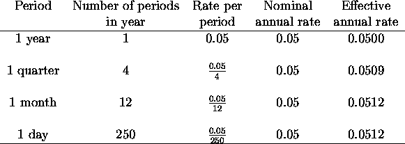
Example, if the annual rate is 5% and this is compounded quarterly
then the rate per quarter is ![]() .
.

Conclusion: you do a little bit better if it is more frequently compounded, but it reaches a limit fast.
In general: have an annual rate r compounded m times a year.
The rate per period is ![]() . How much do you have at the end
of t years?
. How much do you have at the end
of t years?
How many compoundings total? m times a year for t years makes ![]() compoundings. Rate per period is
compoundings. Rate per period is ![]() so the formula gives
so the formula gives
![]()
Now the calculus part: let m get large. That is compound more and more frequently.
Consider the limit:
![]()
Answer:
![]()
So that the number e comes in naturally as a limit in continuous compounding.
Aside: where does this limit come from?
Assume the limit exists, and call it L, then:
![]()
So
![]()
If we are allowed ...
![]()
Now, log of a product is the sum of the logs ...
![]()
Use log rules:
![]()
But as m gets large, so ![]() gets really small, so can use the
log approximation
gets really small, so can use the
log approximation ![]() , to get
, to get
![]()
Cancel to get
![]()
Now exp both sides to get
![]()
Examples: from the old exams.
How long does it take a principal amount to double if the interest rate is
![]() ?
?
Principal is ![]() .
.
Principal has doubled when amount at time t equals twice the principal.
That is ![]() .
.
So the question is, what value of t (how long) makes ![]() double
double ![]() ?
?
The formula for continuous compounding states that ![]() ,
so the question is now ``what value of t makes
,
so the question is now ``what value of t makes ![]() ''?
''?
Some simplifications (trying to get at t):

So the doubling time is ln(2)/r and this does not depend on the
principal ![]() .
.
In particular for r equal to 4% or 0.04 we get ln(2)/0.04 = 17.329.
Always check the answers: Say ![]() is 1000.
is 1000.
Then
![]()
So, it has indeed doubled (up to rounding error).
Next example:
A invests $1000 at 5% per annum continuously compounded.
B invests $200 at 20% per annum continuously compounded.
Questions? Does B ever catch up? How long does it take?
B catches up if the difference between them becomes zero.
Alternatively if the ratio of their amounts becomes 1.
Equality can be expressed as a difference of zero or as a ratio of one.
Draw a picture using a graphing package .
When does it happen: either approximate from the graph or work out explicitly once and for all.
A has at time t, ![]() .
.
B has at time t, ![]() .
.
The equality condition can be stated as:
![]()
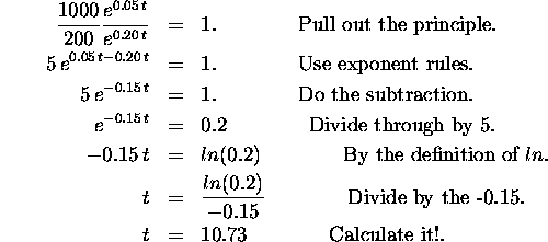
Solve this for t again.

So it takes about 11 years for B to catch up.
Back to the discrete (as opposed to the continuous) case.
After t time intervals, the principal ![]() becomes
becomes
![]()
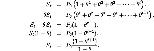
In some instances it is interesting to sum this series, that is
![]()
we can make this look simpler by writing (1 + r) as say ![]() .
Then we have
.
Then we have
![]()
How to find out what ![]() is?
is?

Always check this sort of formula with an example calculation:
Take ![]() ,
, ![]() and t = 3.
and t = 3.
Then
![]()
![]()
![]()
The formula gives
![]()
Language:
The series is: ![]() .
.
The t-th term is ![]() .
.
The sum is ![]() .
.
Recall the formula for the sum of the first t+1 terms is
![]()
What about the limit of this series as ![]() ?
?
Answer is that it depends on the magnitude of ![]() , converges
for
, converges
for ![]() .
.
Geometric series applications: various models as described in the exams. Provides a natural down-weighting, combine various quantities but giving different - higher weight to recent observations - exponential smoothing.
Second part of the class: Functions and straight lines.
Functions: what's the relationship between one variable and another?
Functions express relationships, understanding the relationship means understanding the function.
Three ways to express a functional relationship:
1. Tables.
2. Graphs.
3. Formulae - symbolically.
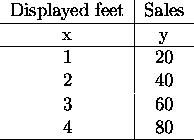
Example: linear feet of shelf space and sales.
Call linear feet ``x'' and sales ``y''.

Graphically: depict a number pair by a point: (1,20),(2,40),(3,60),(4,80).
Draw the point on a graph. the values in the point pairs indicate how far the point is away from a set of axes (in this case 2-axes).
The horizontal axis is called the x-axis, and the vertical is the y axis.
The graph describes a visual description of the relationship.
Formulae Advantage, mathematical objects that can be manipulated
according to a set of rules to provide more information/insight into the
behavior of the relationship. Generically we write y = f(x). In this
example we have ![]() .
.
Straight lines.
The most simple relationship between two variables, and often the level we model at (even if we have to transform to get there, recall Cellular example).
What makes a straight line straight?
The slope of the line is constant.
Slope, the change in y divided by the change in x, ![]() .
.
![]()
Solve to get
![]()
By definition this is true for any values of ![]() and
and ![]() . In particular
. In particular
![]() and just call
and just call ![]() , x.
Get as the equation:
, x.
Get as the equation:
![]()
Terminology: c is the intercept (where the line crosses the y-axis), and m is the slope.
Example: call y the time in seconds to produce x widgets.
![]()
Interpret the slope and intercept.
Intercept: the value of y when x equal zero (in English ...).
Slope, the change in y for every one unit change in x, (in English ...).
Matching up dimensions can provide interpretations.
Question type:
Families of functions.
Homework questions.
A set of quick questions to reinforce the days concepts. A calculator will be needed.