Class 11. Regression for a categorical response

What you need to have learnt from Class 10: Comparing the mean across two categorical variables.

Two basic models:

No interaction: the impact of X1 on Y does not depend on the level of X2.

Interaction: the impact of X1 on Y depends on the level of X2.

Practical consequences:

If NO interaction, then you can investigate the impact of each X by itself.

If there is interaction (consider practical importance as well as statistical significance) then you must consider both X1 and X2 together.

Know and check the assumptions for ANOVA.

New material for today: Regression for a categorical response (logistic regression).

Objective: model a categorical (2-group) response.

Example: how do gender and income impact the probability of the purchase of a product.

Problem: linear regression does not respect the range of the response data (it's categorical).

Solution: model the probability that Y = 1, ie P(Y = 1 | X), in a special way.

Transform P(Y = 1) with the ``logit'' transform.

Now fit a straight line regression to the logit of the probabilities (this respects the range of the data).

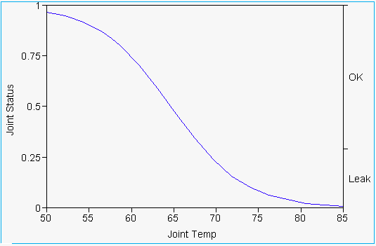
On the original scale (probabilities) the transform looks like this: the curve gives the probability that Y = 1 for a fixed value of X.

The logit is defined as logit(p) = ln(p/(1-p)). Example logit(.25) = ln(.25/(1 - .25)) = ln (1/3) = -1.099.

The three worlds of logistic regression.

The probabilities: this is where most people live. Probability lies in (0,1).

The odds: this is where the gamblers live. Odds lies in (0, Infinity)

The logit: this is where the model lives. Logit lies in (-Infinity, Infinity). Lines lie in (-Infinity,Infinity), therefore fit a line to the logit.

Must feel comfortable moving between the three worlds.

Rules for moving between the worlds. Call P(Y = 1|X), p for simplicity.

logit(p) = ln(p/(1-p))

p = exp(logit(p))/(1 + exp(logit(p))) *** Key to get back to the real world.

odds(p) = p/(1-p)

odds(p) = exp(logit(p)) *** Key for interpretation.

Interpreting the output.

P-values are under the Prob>ChiSq column.

Main equation logit(p) = B0 + B1 X.

B1 = 0. No relationship between X and p.

B1 > 0. As X goes up p goes up.

B1 < 0. As X goes up p goes down.

B1: for every one unit change in X, the ODDS that Y = 1 changes by a multiplicative factor of exp(B1).

At X = -B1/B0 there is a 50% chance that Y = 1.

Key calculation - based on the logistic regression output calculate a probability. Example: Challenger output on p.306.

logit(p) = 15.05 - 0.23 Temp.

Find the probability that Y = 1 (at least one failure) at a temperature of 31.

logit(p) = 15.05 - 0.23 * 31

logit(p) = 7.96.

p = exp(logit(p))/(1 + exp(logit(p)))

p = exp(7.96)/(1 + exp(7.96)) = 0.99965

There is a 99.965 percent chance of at least one failure at a temperature of 31 degrees.