Module 1: Vectors and Workflow
A Motivating Example
In Problem Set 0, we used R to save a single number and perform calculations.
While this functionality may be exciting, we’re ultimately going to be interested in analyzing large amounts of data. Consider the table below which lists different statistics for several basketball players from the 2015-16 NBA regular season. The statistics are:
- field goal makes (FGM)
- field goal attempts (FGA)
- three point makes (TPM)
- three point attempts (TPA)
- free throw makes (FTM)
- free throw attempts (FTA)
| PLAYER | FGM | FGA | TPM | TPA | FTM | FTA |
|---|---|---|---|---|---|---|
| Stephen Curry | 805 | 1597 | 402 | 887 | 363 | 400 |
| John Wall | 572 | 1349 | 115 | 327 | 272 | 344 |
| Jimmy Butler | 470 | 1034 | 64 | 206 | 395 | 475 |
| James Harden | 710 | 1617 | 236 | 657 | 720 | 837 |
| Kevin Durant | 698 | 1381 | 186 | 480 | 447 | 498 |
| LeBron James | 737 | 1416 | 87 | 282 | 359 | 491 |
| Kristaps Porzingis | 498 | 1112 | 126 | 342 | 250 | 280 |
| Dirk Nowitzki | 373 | 886 | 81 | 243 | 201 | 240 |
| Tim Duncan | 215 | 442 | 0 | 2 | 92 | 131 |
| Andre Drummond | 552 | 1061 | 2 | 6 | 208 | 586 |
How are we going to load this data into R?
Vectors
The fundamental unit of data storage in R is a vector, which is simply an ordered collection of data. We can input each column in the above table as a vector. Luckily, many of R’s functions act on these vectors, which allow us to do the same calculation on a lot of different values at once.
Creating vectors
To create a vector containing the field goal makes (FGM), we use the combine function c() and enter each number within the parantheses separated by commas. In the code example below, we create a vector called fgm which contains the FGM statistics from each player in the table and then print it out.
> fgm <- c(805, 572, 470, 710, 698, 737, 498, 373, 215, 552)
> fgm
 [1] 805 572 470 710 698 737 498 373 215 552
Exercise: Create vectors fga, tpm, tpa, ftm and fta which contain the FGA, TMP, TPA, FTM, FTA statistics for each player respectively.
In R, the elements of a vector do not necessarily have to numbers. They can be character strings too. Below, we create a vector that contains the names of the players in the above table.
> players <- c("Stephen Curry", "John Wall", "Jimmy Butler", "James Harden", "Kevin Durant",
+     "LeBron James", "Kristaps Porzingis", "Dirk Nowitzki", "Tim Duncan", "Andre Drummond")
Vectors can also contain what are known as logicals, but we will rarely if ever encounter such vectors in this course. It is important to note, however, that every element of a vector must be of the same type. That is, you cannot have a vector whose first element is a number and whose second element is a character string. Let’s see what happens if we try:
> x <- c(23, "LeBron")In this example, R did not return an error. However, if we print out x, we see that it has coerced the number 23 into a character string ``23 ’’.
Later in the course, we will sometimes need to create a vector of evenly spaced numbers. To do this, we use the seq() command. If we need to create a vector of consecutive integers, we can use the : syntax. Both are demonstrated below
> seq(from = 0, to = 1, by = 0.1)
 [1] 0.0 0.1 0.2 0.3 0.4 0.5 0.6 0.7 0.8 0.9 1.0
> seq(from = 0, to = 1, length = 11)
 [1] 0.0 0.1 0.2 0.3 0.4 0.5 0.6 0.7 0.8 0.9 1.0
> 1:10
 [1]  1  2  3  4  5  6  7  8  9 10
Naming elements in a vector
We’re nearly done loading all of the data into the R. Now, we can start to summarize each column of the data and also start computing new statistics from the ones listed in the table above. Before proceeding, we have one more organizational task.
We know that the first element of the vector fgm is Stephen Curry’s FGM while the ninth element of tpa is the number of three point shots that Dirk Nowitzki attempted. When we print out fgm or tpa for instance, R does not tell us which values correspond to which players.
> fgm
 [1] 805 572 470 710 698 737 498 373 215 552
> tpa
 [1] 887 327 206 657 480 282 342 243   2   6
As we proceed with our analysis, it’ll be useful to have named the elements of the vector. We can do that with the names() function.
> fgm
 [1] 805 572 470 710 698 737 498 373 215 552
> names(fgm) <- players
> fgm
     Stephen Curry          John Wall       Jimmy Butler
               805                572                470
      James Harden       Kevin Durant       LeBron James
               710                698                737
Kristaps Porzingis      Dirk Nowitzki         Tim Duncan
               498                373                215
    Andre Drummond
               552
When we use names(), we put the vector whose elements we want to name in the parantheses and on the right-hand side of the <- we put a character vector of the same length as the vector we want to name containing the element names. In the example above, we set the names of fgm to be the elements of the vector players.
Exercise Name the elements of fga, tpm, tpa, ftm and fta.
Vector Arithmetic
Once we have created a vector, we can perform calculations on each element of the vector with very straightforward syntax:
> fgm + 5
     Stephen Curry          John Wall       Jimmy Butler
               810                577                475
      James Harden       Kevin Durant       LeBron James
               715                703                742
Kristaps Porzingis      Dirk Nowitzki         Tim Duncan
               503                378                220
    Andre Drummond
               557
> fgm/5
     Stephen Curry          John Wall       Jimmy Butler
             161.0              114.4               94.0
      James Harden       Kevin Durant       LeBron James
             142.0              139.6              147.4
Kristaps Porzingis      Dirk Nowitzki         Tim Duncan
              99.6               74.6               43.0
    Andre Drummond
             110.4
> fgm^5
     Stephen Curry          John Wall       Jimmy Butler
      3.380488e+14       6.123224e+13       2.293450e+13
      James Harden       Kevin Durant       LeBron James
      1.804229e+14       1.656827e+14       2.174390e+14
Kristaps Porzingis      Dirk Nowitzki         Tim Duncan
      3.062998e+13       7.220116e+12       4.594014e+11
    Andre Drummond
      5.125018e+13
> sqrt(fgm)
     Stephen Curry          John Wall       Jimmy Butler
          28.37252           23.91652           21.67948
      James Harden       Kevin Durant       LeBron James
          26.64583           26.41969           27.14774
Kristaps Porzingis      Dirk Nowitzki         Tim Duncan
          22.31591           19.31321           14.66288
    Andre Drummond
          23.49468
In each of these examples, we see that arithmetic proceeds elements-wise: fgm + 5 added 5 to every element of fgm while sqrt(fgm) took the square root of every element in fgm.
In basketball, field goal percentage (FGP) is one of the simplest statistic we can use to summarize a player’s ability to shoot the ball well. FGP is defined as FGA/FGM. We can use the vectors fga and fgm to create a new vector fgp that records each players’ field goal percentage.
> fgp <- fgm/fga
> fgp
     Stephen Curry          John Wall       Jimmy Butler
         0.5040701          0.4240178          0.4545455
      James Harden       Kevin Durant       LeBron James
         0.4390847          0.5054308          0.5204802
Kristaps Porzingis      Dirk Nowitzki         Tim Duncan
         0.4478417          0.4209932          0.4864253
    Andre Drummond
         0.5202639
To evaluate fgm / fga, R took the first element of fgm and divided it by the other first element of fga and so on. In order for this to work, fgm and fga had to be the same length. Technically, R is able to handle element-wise arithmetic when the vectors are not of the same length (this is known as recycling) but we will not get into it. For the purposes of this class, whenever you want to do element-wise arithmetic with two vectors, they need to be of the same length.
To determine the length of a vector we can use the function length() as follows:
> length(fgm)
[1] 10
> length(fga)
[1] 10
> length(c(1, 2, 3))
[1] 3
Exercise Create vectors tpp and ftp which contain the three-point percentages (TPP) and free throw percentages (FTP) of the players in the table. If a player’s field goal percentage, three point percentage, and free throw percentage exeed 50%, 40%, and 90%, respectively, they are said to belong to the 50-40-90 club. Did any of the players in the table above qualify for the 50-40-90 club?
Vector Functions
Up to this point, we have seen how to perform element-wise arithmetic with vectors. Now that we have created the vectors fgp, ftp, and tpp we can start to study the distribution of these datasets. R has several functions that operate on entire vectors (i.e. single datasets) but not in an element-wise fashion. Below are a couple of examples. Exercise Try to describe what each of the functions below does
> sum(fgp)
[1] 4.723153
> mean(fgp)
[1] 0.4723153
> sd(fgp)
[1] 0.03931162
> min(fgp)
[1] 0.4209932
> max(fgp)
[1] 0.5204802
> median(fgp)
[1] 0.4704854
> range(fgp)
[1] 0.4209932 0.5204802
> length(fgp)
[1] 10
> sort(fgp)
     Dirk Nowitzki          John Wall       James Harden
         0.4209932          0.4240178          0.4390847
Kristaps Porzingis       Jimmy Butler         Tim Duncan
         0.4478417          0.4545455          0.4864253
     Stephen Curry       Kevin Durant     Andre Drummond
         0.5040701          0.5054308          0.5202639
      LeBron James
         0.5204802
> quantile(fgp)
       0%       25%       50%       75%      100%
0.4209932 0.4412740 0.4704854 0.5050907 0.5204802
> summary(fgp)
   Min. 1st Qu.  Median    Mean 3rd Qu.    Max.
 0.4210  0.4413  0.4705  0.4723  0.5051  0.5205
Indexing
Up to this point, we have created, manipulated, and summarized vectors. To do this, we took advantage of R’s ability to operate on entire vectors at once. But what if we wanted to look at only a few elements of the vectors? For example, what if we wanted to compute the difference in Stephen Curry’s field goal percentage and Dirk Nowitzki’s field goal percentage? To do this, we need a way to extract specific elements of a vector. This is known as subsetting and is an EXTREMELY important aspect of R since it allows us to extract and modify specific elements of an object.
To subset vectors, we will use the single-bracket notation [ ]. Between the brackets we will specify which elements we want to extract. So to extract the first element of fgm we would execute fgm[1] and to extract the third element we would execute fgm[3]:
> fgm[1]
Stephen Curry
          805
> fgm[3]
Jimmy Butler
         470
If you look at the output, you’ll see that when prints the value of fgm[1] or fgm[3], the value is preceded by a [1]. This is R’s way of letting you know that it is printing out a vector. So what is really happening under the hood when we subset a vector is that R is creating another temporary vector containing only the elements we wanted to subset. However, if we look in our environment pane, we see that there is no additional vector, which means that R is not saving that temporary vector. We, of course, could save it using the assignment operator and modify the new vector as much as we want:
> x <- fgm[1]
> y <- x + 3
Above, the first line of code subsets the first element of fgm, creating a temporary vector of length 1 containing the first element of fgm, and saves the result as x. In the next line, it adds three to this value and saves the result as y. Of course, if all we wanted to do was create a vector of length one containing only the value of three plus the first element of fgm, we could have done y <- fgm[1] + 3.
Here we see for the first time an example of R’s order of operations: subsetting happens before operations like addition. We will have a lot more to say about the order of operations a bit later.
We can also use our [ ] syntax to modify vectors. For instance, suppose we made a mistake inputing the first number of fgm, while the rest are fine. We can change this using subsetting:
> fgm[1] <- 105Exercise: Change the first element of fgm back to 805.
We are not limited to subsetting one element at a time. In order to subset multiple elements, we put a vector between the brackets:
> fgm[c(1, 3)]
Stephen Curry  Jimmy Butler
          805           470
> fgm[1:2]
Stephen Curry     John Wall
          805           572
> players[c(1, 3)]
[1] "Stephen Curry" "Jimmy Butler"
We can also use names to subset vectors. Instead of putting a number (or vector of numbers) between the bracket, we now put a character string (or vector of character strings) specifying the names of vector elements we want to subset.
> fgp["Stephen Curry"]
Stephen Curry
    0.5040701
> fgp[c("Stephen Curry", "Dirk Nowitzki")]
Stephen Curry Dirk Nowitzki
    0.5040701     0.4209932
> fgp["Stephen Curry"] - fgp["Dirk Nowitzki"]
Stephen Curry
    0.0830769
NBA Shooting Metrics
Of the ten players in the table above, we see that LeBron James had the highest field goal percentage. As it turns out, during the 2015–16 season, DeAndre Jordan led the league in field goal percentage, making just over 70% of his shots. Meanwhile, Steph Curry made just over 50% of his shots. Does this mean that DeAndre Jordan is the better shooter than Curry?
One criticism of FGP is that it treats 2-point shots the same as 3-point shots. As a result, the league leader in FGP is usually a center whose shots mostly come from near the rim. effective Field Goal Percentage is a statistic that adjusts FGP to account for the fact that a made 3-point shots is worth 50% more than a made 2-point shot. The formula for eFGP is \[ \text{eFGP} = \frac{\text{FGM} + 0.5 \times \text{TPM}}{\text{FGA}}.\] We can compute the effective field goal percentage of all ten players as follows
> efgp <- (fgm + 0.5 * tpm)/fga
> efgp
     Stephen Curry          John Wall       Jimmy Butler
         0.6299311          0.4666420          0.4854932
      James Harden       Kevin Durant       LeBron James
         0.5120594          0.5727734          0.5512006
Kristaps Porzingis      Dirk Nowitzki         Tim Duncan
         0.5044964          0.4667043          0.4864253
    Andre Drummond
         0.5212064
We see now that Curry has the highest effective field goal percentage. Before declaring Curry was the best shooter out of these ten players, though, we might pause and ask about free throws. Both field goal percentage and effective field goal percentage totally ignore free throws. One metric that accounts for all field goals, three pointers, and free throws is true shooting percentage, whose formula is given by \[ \text{TPS} = \frac{\text{PTS}}{2\times(\text{FGA} + 0.44\times \text{FTA})}, \] where \(\text{PTS} = \text{FTM} + 2 \times \text{FGM} + \text{TPM}\) is the number of points scored.
Exercise Create vectors pts and tsp for points scored (PTS) and true shooting percentage (TSP). Which player had the highest true shooting percentage?
R Scripts
Up to this point, we have been working strictly within the R console, proceeding line-by-line. As our commands become more and more complex, you’ll find that using the console can get pretty cramped. And if you make a mistake in entering your code, you’ll get an error and have to start all over again. Plus, when we start a new session of R Studio, the console is cleared. How can we save the commands we typed into R? We do so using an R Script. An R Script is a file type which R recognizes as storing R commands and is saved as a .R file. R Scripts are useful as we can edit our code before sending it to be run in the console.
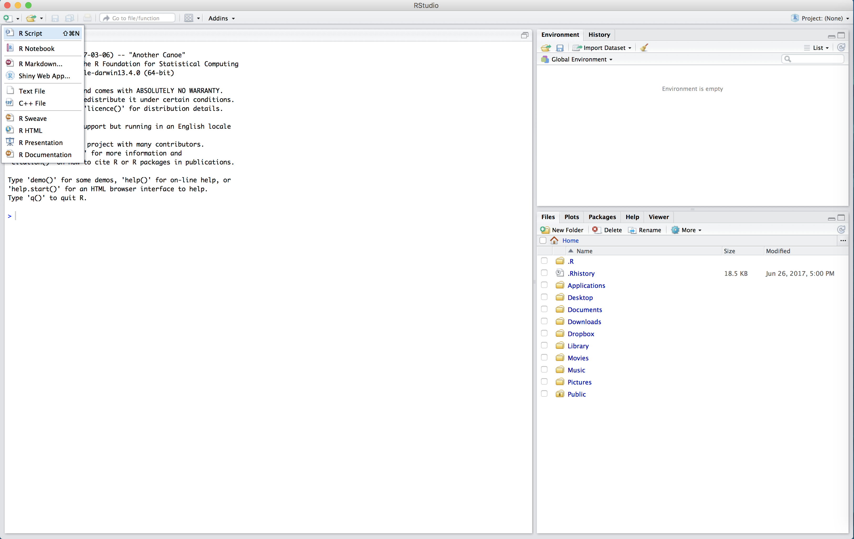
We can start a new R Script by clicking on the top left symbol in R Studio and selecting “R Script”.
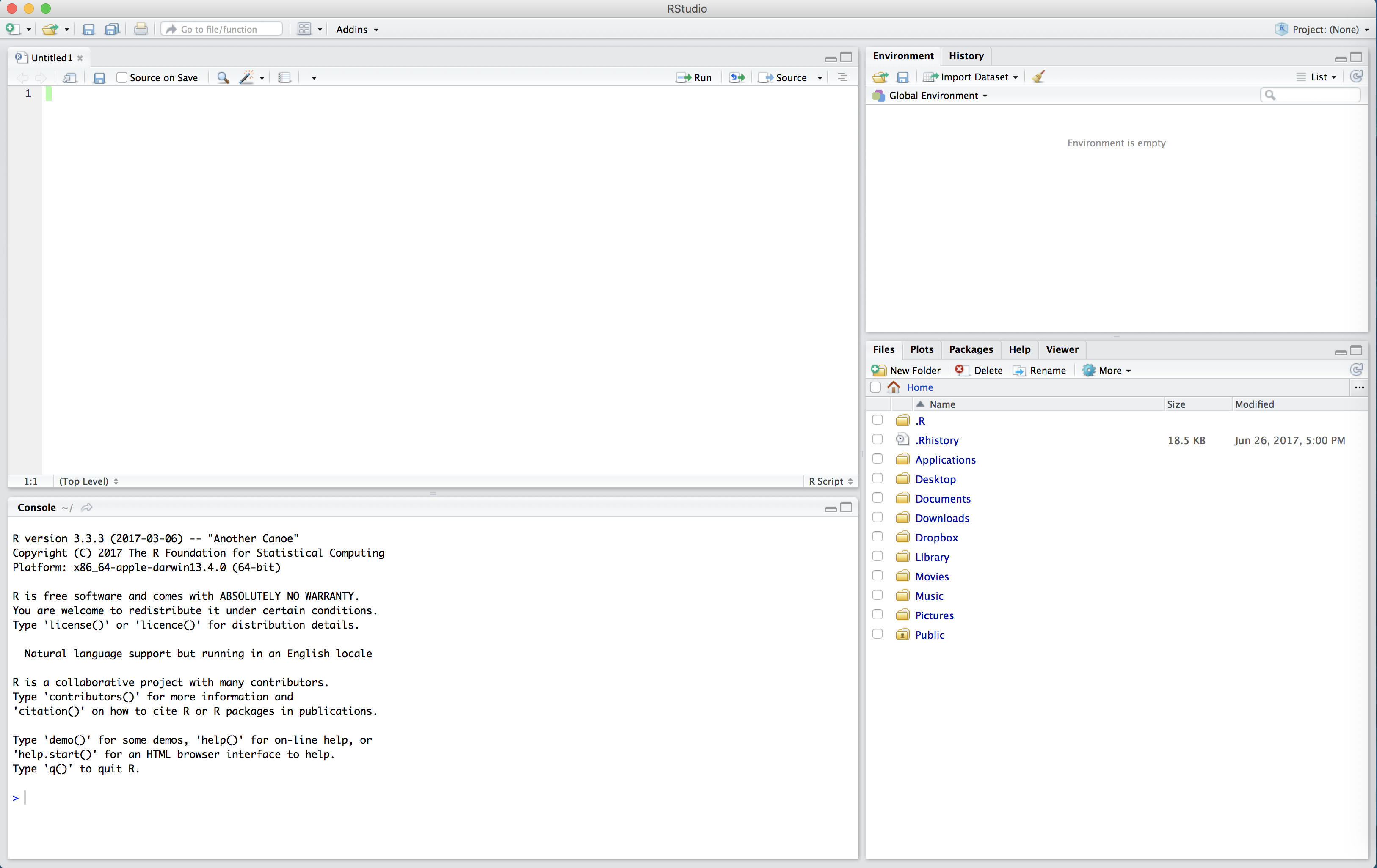
The untitled R Script will then appear in the top left hand box of R Studio.
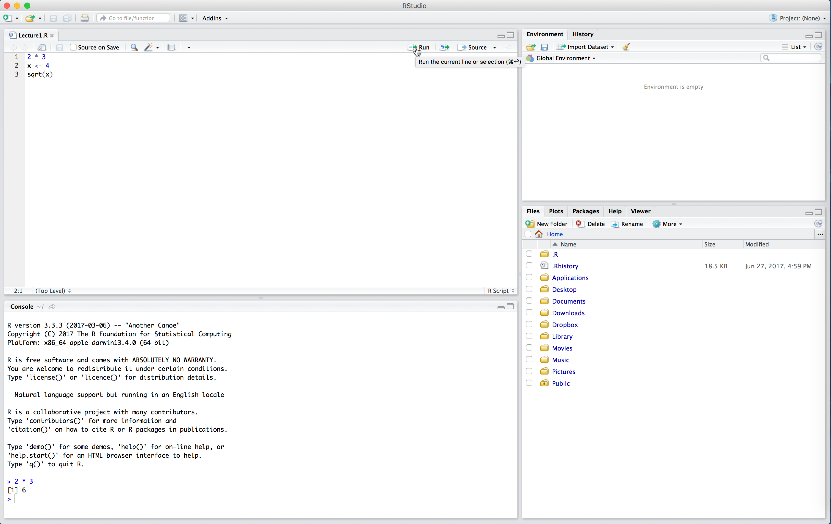
In the R Script, type the following:
2 * 3
x <- 4
sqrt(x)
Now our code is just sitting in the R Script. To run the code (that is, evalutate it in the console) we click the “Run” button in the top right of the script. This will run one line of code at a time - whichever line the cursor is on. Place your cursor on the first line and click “Run”. Observe how 2 * 3 now appears in the console, as well as the output 6.
If we want to run multiple lines at once, we highlight them all and click “Run”.
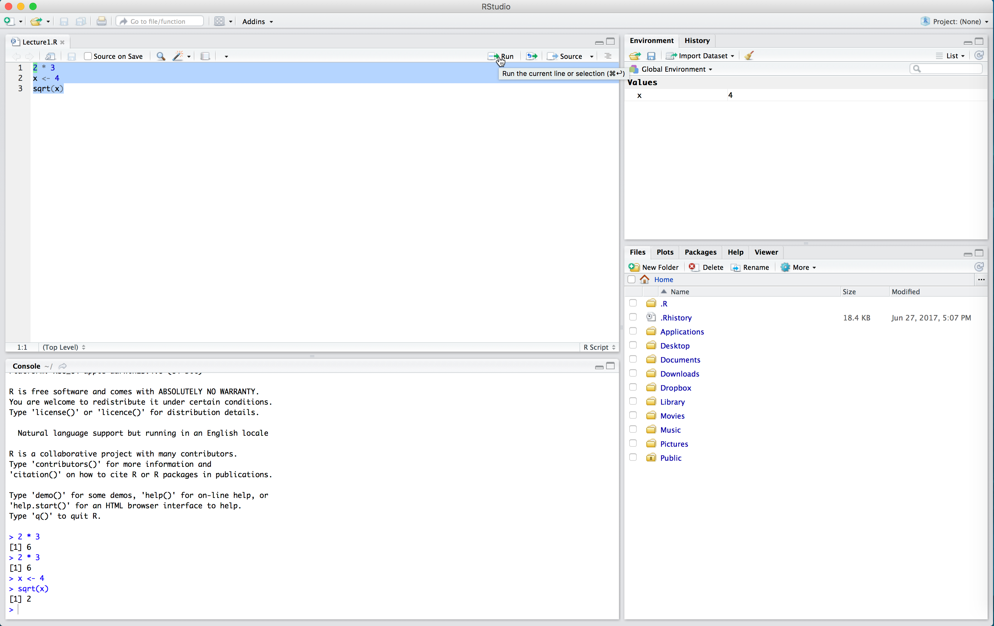
Note in the above that we had to run x <- 4 before sqrt(x). We need to define our variables first and run this code in the console before performing calculations with those variables. The console can’t “see” the script unless you run the code in the script.
One very nice thing about RStudio’s script editor is that it will highlight syntax errors with a red squiggly line and a red cross in the sidebar. If you move your mouse over the line, a pop-up will appear that can help you diagnose the potential problem.
Another advantage of R scripts is thta you can add comments to your code, which are preceded by the pound sign / hash sign #. Comments are useful because they allow you to explain what your code is doing.
Exercise Create a new R script called “module1.R”" which contains all of the code used to load the data from the table above and computing all of the vectors of shooting statistics. Be sure to add some comments!