26 Analysis of Variance
Rather than use a special tool, a one-way analysis of variance is easily estimated in R as a multiple regression that has one categorical explanatory variable. R also has a special function for ANOVA models as well. The new tools in this chapter include
orderedspecifies the order for the categories of a factoraovbuilds a regression model for the analysis of varianceTukeyHSDperforms Tukey comparisons of group means
26.1 Analytics in R: Judging the Credibility of Advertisements
The data file for this example contains the response, the credibility assigned to an advertisement, and a categorical explanatory variable that identifies nature of the claims made in the ad. We do not need the dummy variables that are included in the data file; R will build those as part of the regression model.
Ads <- read.csv("Data/26_4m_credibility.csv")
dim(Ads)
## [1] 80 5head(Ads)## Credibility Treatment D_Plausible D_Stretch D_Outrageous
## 1 1.3 Tame 0 0 0
## 2 -1.4 Tame 0 0 0
## 3 -0.7 Tame 0 0 0
## 4 -0.7 Tame 0 0 0
## 5 -2.3 Tame 0 0 0
## 6 6.8 Tame 0 0 0There are four categories of exaggeration in the shown ads, with 20 cases in each group. (The experiment is balanced, having an equal number of cases in each group.)
table(Ads$Treatment)##
## Outrageous Plausible Stretch Tame
## 20 20 20 20lm builds dummy variables for 3 categories of the variable Treatment, omitting the first category alphabetically (“Outrageous”).
regr <- lm(Credibility ~ Treatment, data=Ads)
regr
##
## Call:
## lm(formula = Credibility ~ Treatment, data = Ads)
##
## Coefficients:
## (Intercept) TreatmentPlausible TreatmentStretch
## -2.995 2.530 2.925
## TreatmentTame
## 3.655To get results like those in the text (which leaves out the last category alphabetically), replace the unordered factor in the data table by an ordered factor. By ordering the categories, you can control which category is the “baseline” group that is not represented by a dummy variable.
Ads$Treatment <- ordered(Ads$Treatment,
                         levels=c("Tame","Plausible","Stretch","Outrageous"))
Now because the category “Tame” is the first category, it will form the baseline group. We also need to set an obscure option to get the estimates associated with dummy variables. (Otherwise R will use polynomial contrasts when a model includes an ordered factor.)
options(contrasts= c('contr.treatment', 'contr.treatment'))

regr <- lm(Credibility ~ Treatment, data=Ads)
summary(regr)
##
## Call:
## lm(formula = Credibility ~ Treatment, data = Ads)
##
## Residuals:
## Min 1Q Median 3Q Max
## -9.4300 -2.0412 0.1175 2.3125 8.9700
##
## Coefficients:
## Estimate Std. Error t value Pr(>|t|)
## (Intercept) 0.6600 0.8754 0.754 0.4532
## TreatmentPlausible -1.1250 1.2381 -0.909 0.3664
## TreatmentStretch -0.7300 1.2381 -0.590 0.5572
## TreatmentOutrageous -3.6550 1.2381 -2.952 0.0042 **
## ---
## Signif. codes: 0 '***' 0.001 '**' 0.01 '*' 0.05 '.' 0.1 ' ' 1
##
## Residual standard error: 3.915 on 76 degrees of freedom
## Multiple R-squared: 0.115, Adjusted R-squared: 0.08005
## F-statistic: 3.291 on 3 and 76 DF, p-value: 0.02506The residuals appear to have similar variation across the 4 groups. (With 4 rather than 2 groups in a two-sample t-test, you expect larger differences among the interquartile ranges due to random variation.)
boxplot(residuals(regr) ~ Ads$Treatment)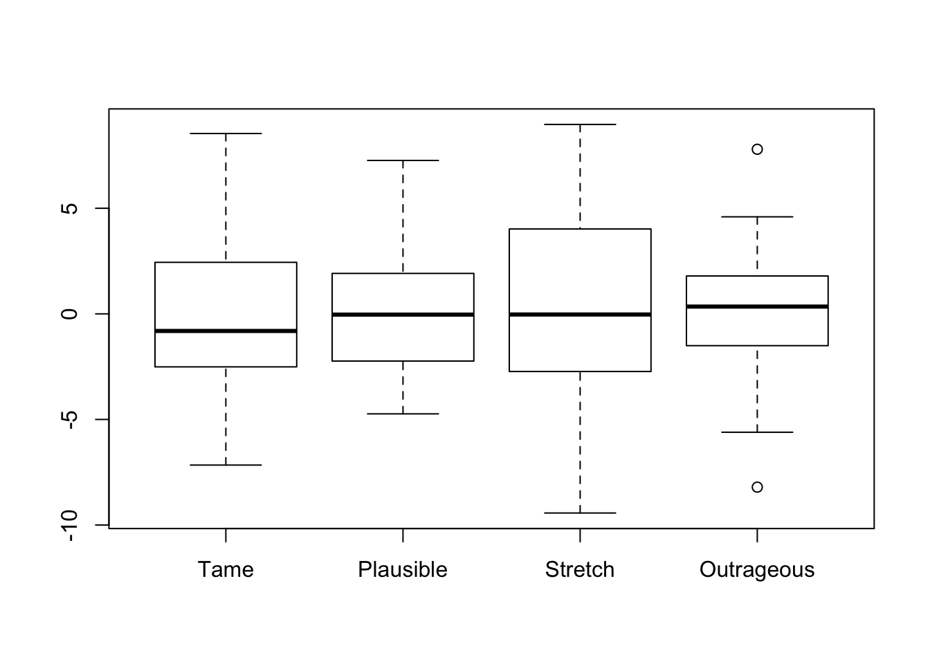
If you only want the mean within each group, tapply is easier to use.
tapply(Ads$Credibility, Ads$Treatment, mean)## Tame Plausible Stretch Outrageous
## 0.660 -0.465 -0.070 -2.995In order to get Tukey multiple comparisons, you need to first build an anova object. The syntax of the function aov for specifying the variables in the model is exactly the same as that when using lm.
model <- aov(Credibility ~ Treatment, data=Ads)
model
## Call:
## aov(formula = Credibility ~ Treatment, data = Ads)
##
## Terms:
## Treatment Residuals
## Sum of Squares 151.3505 1164.9250
## Deg. of Freedom 3 76
##
## Residual standard error: 3.915094
## Estimated effects may be unbalancedTo get the estimated coefficients (notice the default order), use the function coefficients. These are the same estimates as in the regression with the ordered factor.
coefficients(model)## (Intercept) TreatmentPlausible TreatmentStretch
## 0.660 -1.125 -0.730
## TreatmentOutrageous
## -3.655R does not produce standard errors for these as in a regression. To get those, feed this model into the function TukeyHSD. The output of TukeyHSD is a list of all pairwise comparisons among the four groups. For each comparison, the output shows the difference between the pair of means, the endpoints of the 95% confidence interval for the difference, and a p-value for testing \(H_0\) that the means are the same. In this example, only the comparison of the credibility of “Outrageous” ads to “Tame” ads is statistically significant. The p-value for this comparison 0.02138 < 0.05 and the confidence interval for the difference [-6.907 -0.403] does not include zero.
TukeyHSD(model) ## Tukey multiple comparisons of means
## 95% family-wise confidence level
##
## Fit: aov(formula = Credibility ~ Treatment, data = Ads)
##
## $Treatment
## diff lwr upr p adj
## Plausible-Tame -1.125 -4.377136 2.1271356 0.8002689
## Stretch-Tame -0.730 -3.982136 2.5221356 0.9349251
## Outrageous-Tame -3.655 -6.907136 -0.4028644 0.0213802
## Stretch-Plausible 0.395 -2.857136 3.6471356 0.9886768
## Outrageous-Plausible -2.530 -5.782136 0.7221356 0.1813905
## Outrageous-Stretch -2.925 -6.177136 0.3271356 0.0932426