15 Confidence Intervals

It is simple to compute confidence intervals once you have the summary statistics \(\overline{X}\) and \(S\). Software in R provides these easily and removes the need to use tables for percentiles of the normal or t-distributions. The R functions specifically illustrated in this chapter are:

• qt find quantiles of the t-distribution
• round rounds the endpoints of confidence intervals to more useful numbers of digits
• qnorm finds the quantiles of the normal distribution

15.1 Analytics in R: Property Taxes

Start by reading the data file. The data give the cost of a lease, in dollars, for 223 properties in the city under study.

Tax <- read.csv("Data/15_4m_property_tax.csv")
dim(Tax)

## [1] 223   1

head(Tax)

##   Total.Lease.Cost
## 1           329959
## 2           298073
## 3          2820213
## 4           883773
## 5           359745
## 6           776486

The distribution of the lease costs is right-skewed.

hist(Tax$Total.Lease.Cost, breaks=12)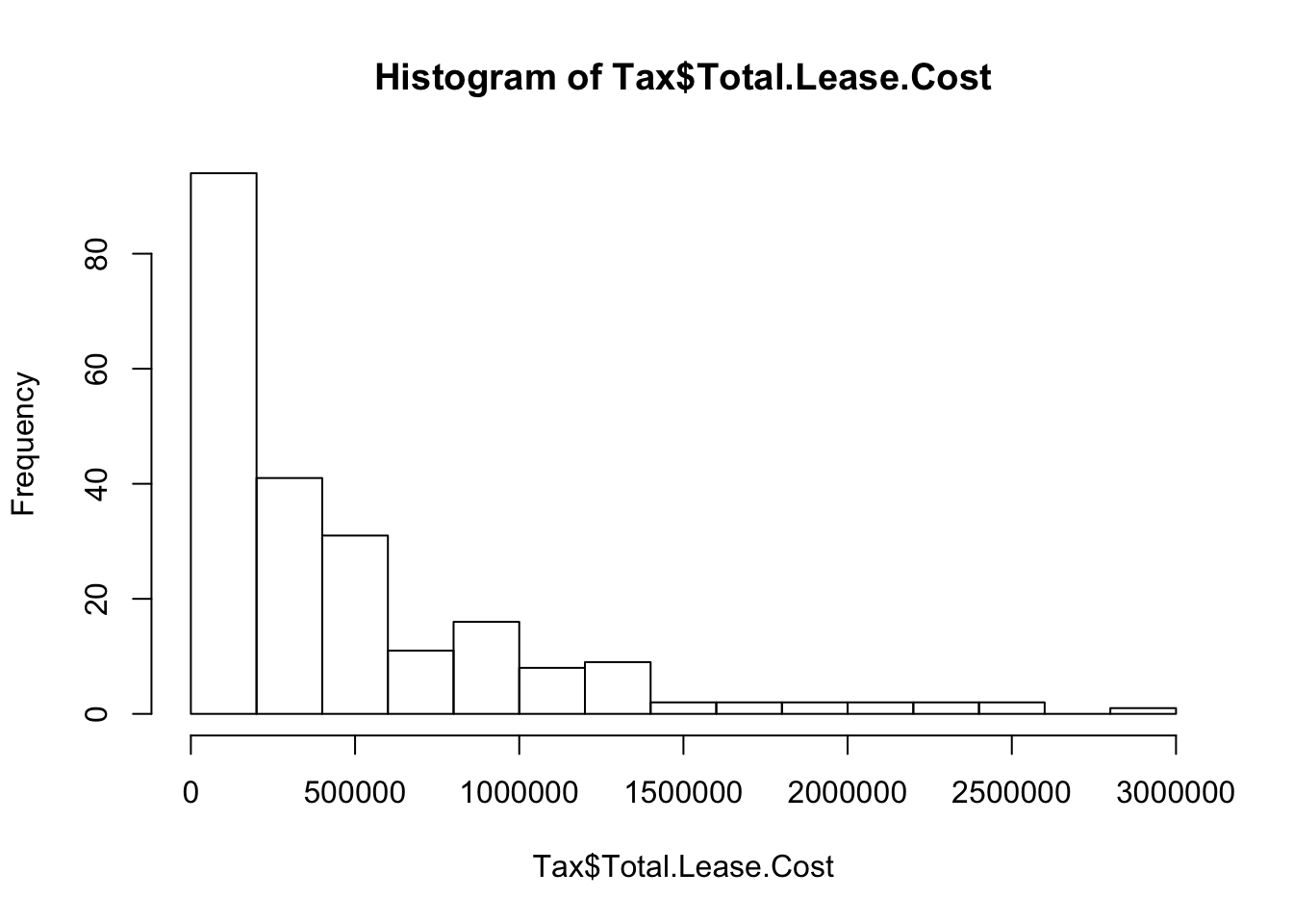

Use the excess kurtosis to check the sample size condition (see Chapter 12).

require(moments)

kurtosis(Tax$Total.Lease.Cost)-3

## [1] 4.018534

The excess kurtosis implies our sample needs to have more than 40 cases in order to rely on averaging to produce approximately normally distributed sampling variation. With \(n=223\) we have more than enough.

Rather than use long expressions when forming a confidence interval, compute the needed statistics first.

n    <- length(Tax$Total.Lease.Cost)
xbar <- mean(Tax$Total.Lease.Cost)
s    <- sd(Tax$Total.Lease.Cost)

Then use the built-in t-distribution to find the needed quantile. Notice the negative sign of the value returned by qt(0.025). You need to change the sign because qt returns the lower 2.5 percentile of the t-distribution, which is negative. The value is slightly less than 2 in absolute size (but larger than 1.96, the “exact” value for the normal distribution). You can avoid the negative sign by asking for the 1-0.025=0.975 quantile, but that seems more difficult to me.

tstat <- - qt(0.025, df=n-1)
tstat

## [1] 1.970707

By making a vector with \(-t_{\alpha/2,n-1}\) and \(t_{\alpha/2,n-1}\), R returns the confidence interval as a 2-element vector with the lower and upper endpoints of the confidence interval.

ci <- xbar + c(-tstat,tstat) * s/sqrt(n)
ci

## [1] 407955.2 549251.7

If like me you make careless errors when rounding the endpoints, you can let R do that for you as well. Specifying -3 digits rounds to the nearest $1000.

round(ci, digits=-3)

## [1] 408000 549000

15.2 Analytics in R: A Political Poll

R can seem like an extensive calculator. We are given \(\hat{p}=0.4\), with \(n = 400\).

phat  <- 0.4
n     <- 400

zstat <- -qnorm(0.025)

ci <- phat + c(-zstat, zstat) * sqrt(phat*(1-phat)/n)
ci

## [1] 0.3519909 0.4480091

Rounding to two decimal places (the nearest multiple of 0.01) seems about right.

round(ci,2)

## [1] 0.35 0.45