2 Data
The data sets used in this book are organized as tables that resemble an Excel spreadsheet. You can enter data directly into R, but most often you will read it from a file. All of the data sets used for the examples in Statistics for Business are available in CSV files. This supplement barely scratches the surface of show what R is capable of doing when it comes to reading data and preparing data for an analysis. You’ll want to read more – a lot more – if you start using R frequently.
Important functions discussed in this chapter are:
read.csvreads CSV files into a data framedimgives the dimensions of a matrix or data framestrandsummaryshow summary information about the columns of data frameheadshows the first six rows of a data frame or R matrix (six elements of a vector)Viewopens a spreadsheet view of a data framewithallows access to columns of a data frame in subsequent commandsinstall.packagesdoes what its name implies: it installs supplemental R code on your computerrequireaccesses extensions to the standard R set of commands as needed
For example, the command read.csv reads a small file that has the bicycle data table shown in the text Table 2.1 (3rd edition version). R puts data such as these into an object called a data frame. The function read.csv returns a data frame. A data frame is a rectangular table that allows you to mix character variables such as the name of the customer, with numerical data, such as sizes or amounts.
Bike <- read.csv("Data/02_bike_shop.csv")
dim(Bike)
## [1] 4 7The function dim (short for “dimensions”) tells us that this data frame has 4 rows and 7 columns. Each row of this data table describes a purchased item at the bike shop.
The function str (short for “structure”) reveals a bit more about those columns, giving the names of the columns and a peek into the contents of each.
str(Bike)## 'data.frame': 4 obs. of 7 variables:
## $ Customer : Factor w/ 3 levels "Bob","Karen",..: 3 2 2 1
## $ Club.Member: int 0 1 1 1
## $ Date : int 52215 6315 61515 82115
## $ Type : Factor w/ 3 levels " Ti"," Tu","B": 3 2 1 3
## $ Brand : Factor w/ 4 levels " Colnago"," Conti",..: 1 2 4 3
## $ Size : int 58 27 27 56
## $ Amount : num 4625 4.5 31.1 3810The function summary (which is chameleon-like and changes behavior from situation to situation) provides a more statistically oriented summary. (Albeit, one that is hardly needed for this tiny data table.)
summary(Bike)## Customer Club.Member Date Type Brand
## Bob :1 Min. :0.00 Min. : 6315 Ti:1 Colnago :1
## Karen:2 1st Qu.:0.75 1st Qu.:40740 Tu:1 Conti :1
## Oscar:1 Median :1.00 Median :56865 B :2 Kestrel :1
## Mean :0.75 Mean :50540 Michelin:1
## 3rd Qu.:1.00 3rd Qu.:66665
## Max. :1.00 Max. :82115
## Size Amount
## Min. :27.0 Min. : 4.50
## 1st Qu.:27.0 1st Qu.: 24.41
## Median :41.5 Median :1920.53
## Mean :42.0 Mean :2117.64
## 3rd Qu.:56.5 3rd Qu.:4013.75
## Max. :58.0 Max. :4625.00Notice from the output of str that R represents categorical variables as objects called factors. A factor is another, often-confusing-when-first met historical legacy that persists in R. The original motivation for representing categorical data as factors was to save precious computer memory. Rather than save lots and lots of repeated character strings, a factor in R keeps a list of the unique strings and stores the indices of these. Instead of storing the literal names “Oscar”, “Karen”, “Karen”, and “Bob”, R does the following. R first sorts a list of the unique strings in the column into alphabetical order, here “Bob”, “Karen”, and “Oscar”. Rather than store strings, a factor records which strings appear in the data. “Oscar” comes first, then “Karen”. So, R stores the indices 3, 2, 2, 1 in place of the strings. No, this doesn’t make much sense for a small example, but if these 4 names were repeated thousands of times, the advantage becomes apparent (though still a bit confusing in this age of cheap computer memory).
The data table is small enough to print here. Notice that R doesn’t allow spaces within the name of a column. When a space is encountered (see the name “Club Member” found in the header line of the CSV file), R replaces the space with a “.”.
Bike # R will print the first few lines of a large data table## Customer Club.Member Date Type Brand Size Amount
## 1 Oscar 0 52215 B Colnago 58 4625.00
## 2 Karen 1 6315 Tu Conti 27 4.50
## 3 Karen 1 61515 Ti Michelin 27 31.05
## 4 Bob 1 82115 B Kestrel 56 3810.00The function View presents an interactive spreadsheet view of the data. (Unlike most functions in R, the name of this function begins with a capital letter.) Scroll bars are available when viewing larger tables, and you can interactively sort and filter columns as in Excel.
View(Bike)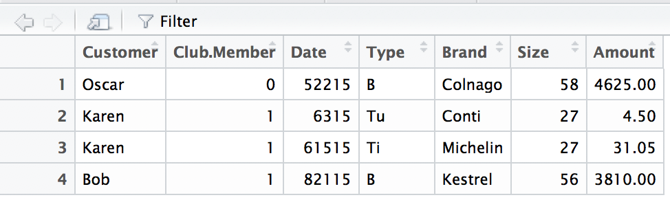
For instance, the first row shows that Oscar, who is not a club member, bought a 56 cm (the size) Colnago bike on May 22, 2015 for $4,625. Notice that I had to know more than what is given in the CSV file to interpret the values in the file. The CSV file doesn’t tell me that 52216 is a date; that’s the extra contextual information that I need to interpret this value. Numbers without context are not data. Similarly, those values in the size column and abbreviations in the type column need context, too.
There are several ways to extract variables from a data frame. One method is to use $ indexing; the syntax requires the name of the data frame, a dollar sign, and then the name of the desired column. For example, this command extracts the amounts:
Bike$Amount## [1] 4625.00 4.50 31.05 3810.00Alternatively, we can treat a data frame as a two-way table and use [ row , column ] indexing like that used to identify elements of a matrix. For example, the value the 2nd row, 6th column of the Bike data frame is
Bike[2,6]## [1] 27and the value in the 4th row, 5th column is
Bike[4,5]## [1] Kestrel
## Levels: Colnago Conti Kestrel MichelinWhen showing an element of a factor, R lists all of the possible labels below the found value.
You can use bracket indexing to extract a column (aka, a variable). If you omit one of the indices, you get a whole column or row.
Bike[1,] # first row## Customer Club.Member Date Type Brand Size Amount
## 1 Oscar 0 52215 B Colnago 58 4625Bike[,3] # third column## [1] 52215 6315 61515 82115You can also identify columns of a data frame by name when using the bracket style of indexing,
Bike[,"Date"]## [1] 52215 6315 61515 82115That’s the same as the more easily typed
Bike$Date## [1] 52215 6315 61515 821152.1 Dates and Time Series
Dates are important in data, and R has special functions for handling them in order to get sensible results and plots. As an example, this command builds a data frame with the monthly unemployment data shown in Figure 2.2.
Unemp <- read.csv("Data/02_unempl.csv")
dim(Unemp)
## [1] 816 3The head command shows the first 6 rows of a data frame. That’s better than looking at the entire file. (Notice that once again R replaced blanks in the column names by dots.)
head(Unemp)## Calendar.Date Unemployment.Rate Date
## 1 01/01/1948 3.4 1948.000
## 2 02/01/1948 3.8 1948.083
## 3 03/01/1948 4.0 1948.167
## 4 04/01/1948 3.9 1948.250
## 5 05/01/1948 3.5 1948.333
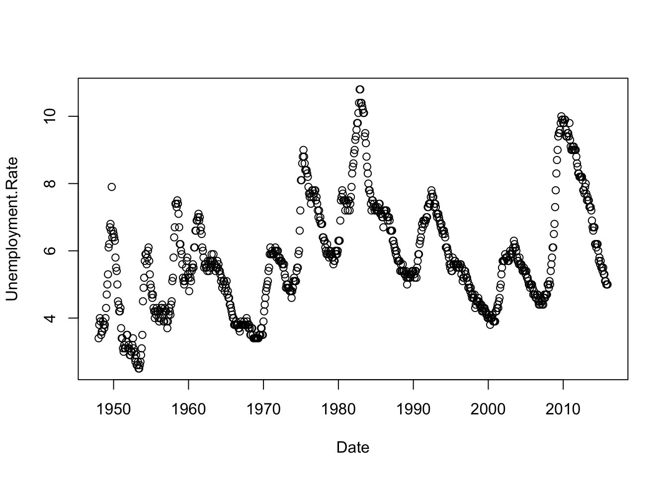
## 6 06/01/1948 3.6 1948.417The variable Date uses a numbering scheme to produce an x-axis for sequence plots. Let’s generate a sequence plot like that shown in Figure 2.2. When working with a data frame, it is often helpful to use the R function with to avoid having to type the name of the data frame repeatedly. By default, R shows points rather than lines.
with(Unemp,
     plot(Date, Unemployment.Rate)
)
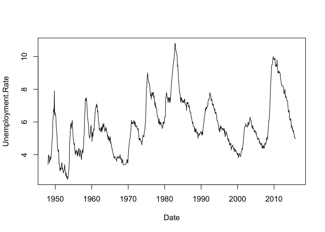
By adding an optional argument to the plot command, we get lines in place of points.
with(Unemp,
     plot(Date, Unemployment.Rate, type='l')    # type='l' means to connect the dots
)
Manipulating dates in R can be tedious, so I use the package lubridate to simplify some of those chores. (Notice that the column Calendar.Date is a factor.) Here’s an example that avoids needing to convert those dates into numbers. Curiously, the number of labels on the x-axis also changes. (You may need to install lubridate using the command install.packages("lubridate"). See the help information in R for more information or use the Packages tab found in the lower right panel of R-Studio.)
require(lubridate)

with(Unemp,
     plot(mdy(Calendar.Date), Unemployment.Rate, type='l')   # mdy = month, day, year
)
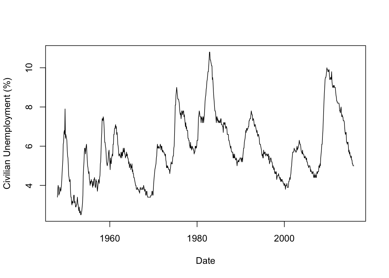
If you’d like better labels on the plot, use the optional arguments xlab and ylab.
with(Unemp,
     plot(mdy(Calendar.Date), Unemployment.Rate, type='l',
          xlab="Date", ylab="Civilian Unemployment (%)")
)
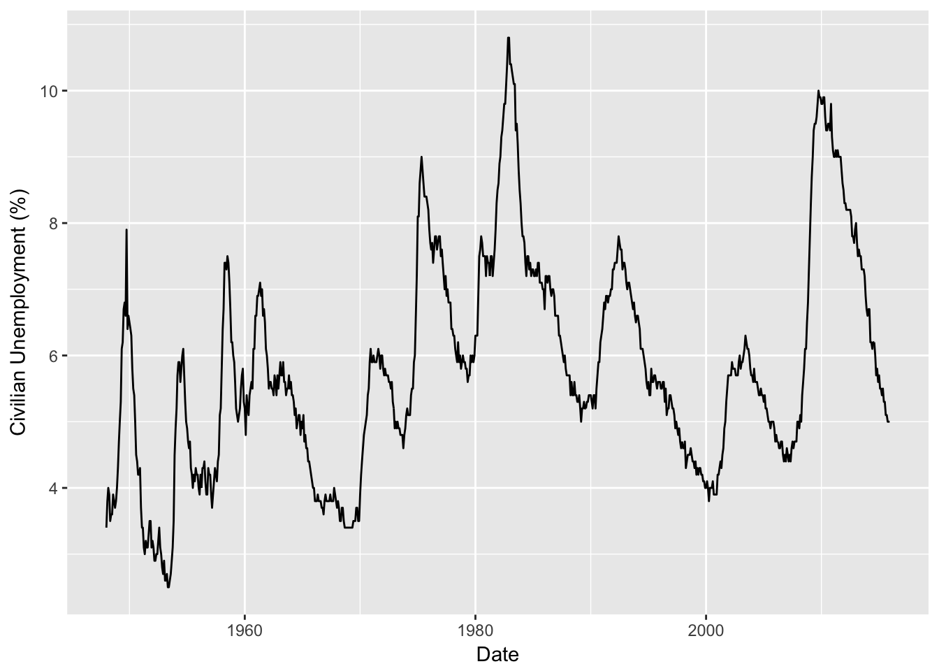
Now that I have mentioned optional packages in R, you might also want to explore ggplot2 which has become very popular. Here’s an example. Although the syntax of ggplot is very different from the default R plot command, you can see that the same information is needed. (Again, you may need to install ggplot2 first in the same way you installed lubridate.)
require(ggplot2)

ggplot(Unemp) +
    geom_line(aes(x=mdy(Calendar.Date), y=Unemployment.Rate)) +
    xlab("Date") + ylab("Civilian Unemployment (%)")