11 Probability Models for Counts
R becomes more useful for the exercises in this chapter because it has built-in functions for a wide range of probability models, including both the binomial and Poisson models for random variables described in this chapter. For each family of random variables, R includes three types of functions, identified by the leading letter:
- the probability distribution (or density function, starting with “d”),
- the cumulative probability distribution (starting with “p”), and
- the quantile function (starting with “q”).
For example, dbinom computes a binomial probability distribution \(P(X = x)\), pbinom the cumulative distribution \(P(X \le x)\), and qbinom the quantiles (a.k.a. percentiles). Given a probability \(p\), the quantile function finds the value \(x\) such that \(P(X \le x) = p\). Similarly, dpois, ppois, and qpois compute these functions for a Poisson random variable. (R defines such functions for many other random variables, such as t-distributions and chi-squared distributions.)
To draw the density function of a discrete random variable like the binomial, the textbook presents the density in the “tethered balloon” style illustrated in R in Chapter 8. For example, here’s the probability distribution of a binomial random variable with parameters \(n = 20\) trials and \(p = 0.25\). The number of trials is specified in R by the size argument.
x <- 0:20
p_x <- dbinom(x, size=20, prob=0.25)             # P(X = x)
plot  (x, p_x, col='gray', type='h', bty='L', ylab="Binomial(20,0.25)")
points(x, p_x, pch=19)                        # solid circle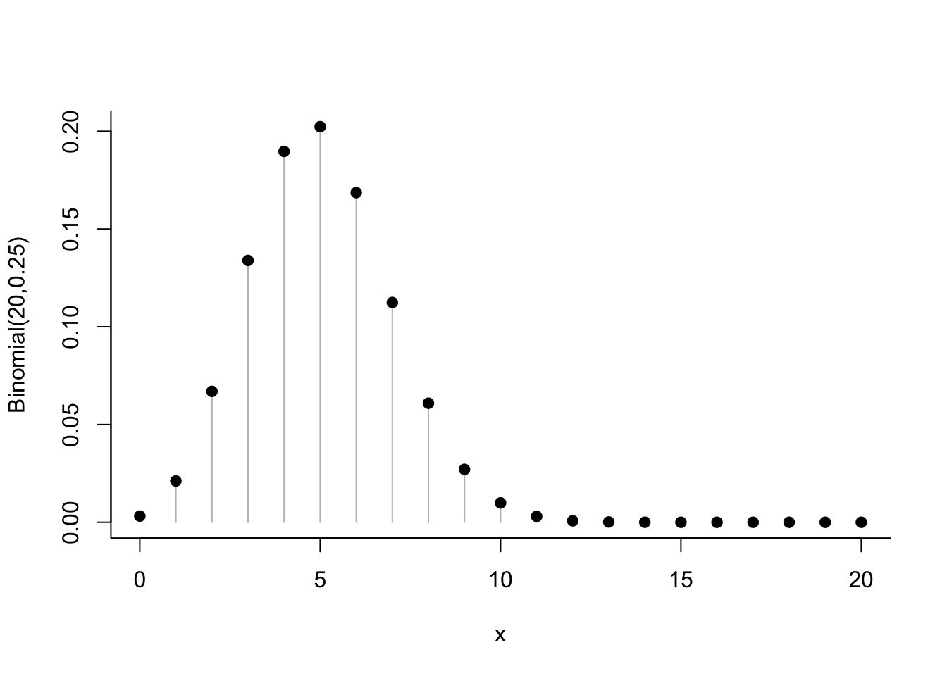
R also has a convenient way to draw the cumulative distribution. This function is tricky to draw otherwise because of the vertical jumps at the integers. (I would prefer that R omit the vertical line at the jump points, but that’s not what it does.)
x   <- 0:20
P_x <- pbinom(x, size=20, prob=0.25)    # P(X <= x)
plot  (x, P_x , type='s', bty='L', ylab="Binomial(20,0.25)")
points(x, P_x, pch=18)               # diamond shaped point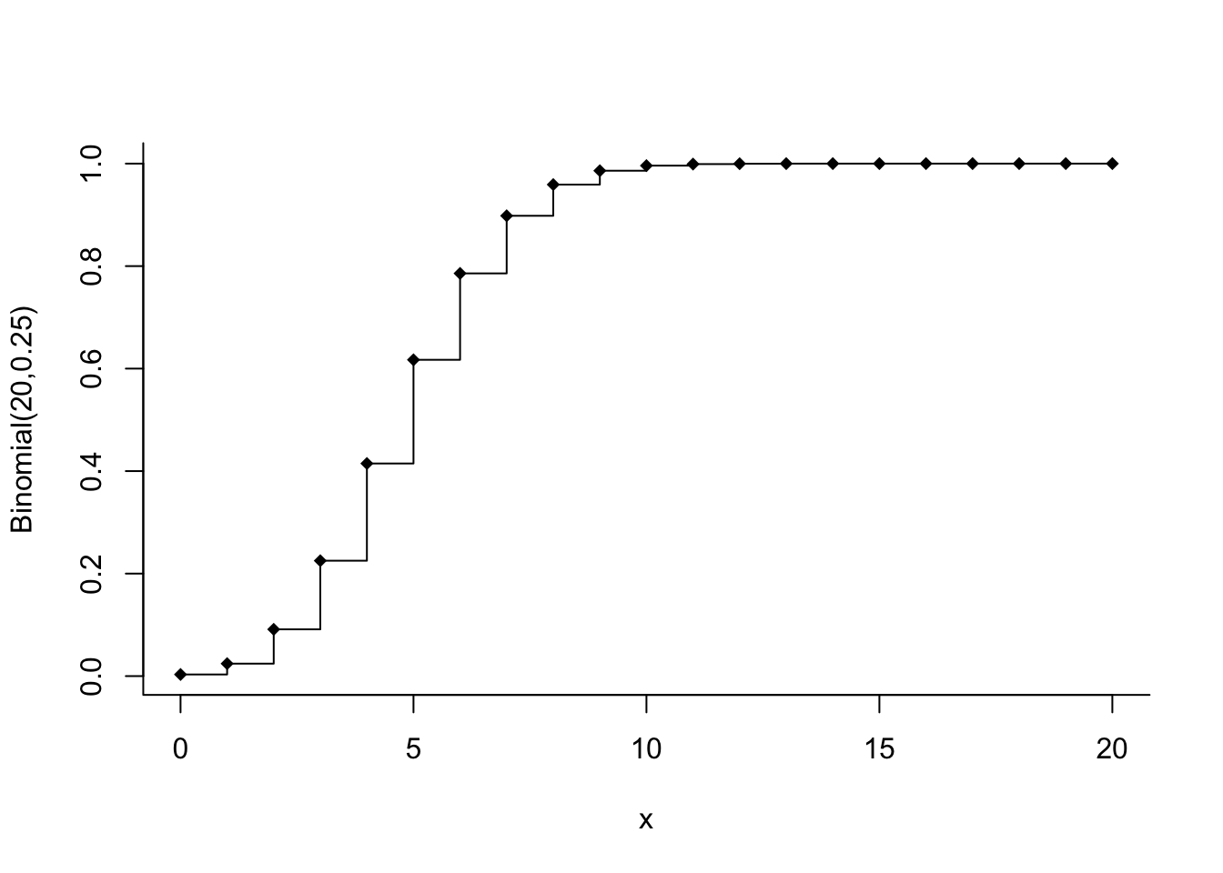
To see other choices for drawing points, look at the help information given for pch.
11.1 Analytics in R: Focus on Sales
The random variable is \(Y \sim Bi(n=9, p=0.8)\). Here’s the probability distribution of \(Y\), first listed in a table and then shown in a plot.
y   <- 0:9                          # possible values of the r.v.
p_y <- dbinom(y, size=9, prob=0.8)     # P(Y = y)
To show these neatly as a table, join the two vectors side by side to form a matrix, then assign names to the columns of the matrix.
dist <- cbind(y,p_y)
colnames(dist) <- c("y", "p(y)")
dist
## y p(y)
## [1,] 0 0.000000512
## [2,] 1 0.000018432
## [3,] 2 0.000294912
## [4,] 3 0.002752512
## [5,] 4 0.016515072
## [6,] 5 0.066060288
## [7,] 6 0.176160768
## [8,] 7 0.301989888
## [9,] 8 0.301989888
## [10,] 9 0.134217728plot(y, p_y, type='h', col='gray', bty='l')
points(y,p_y, pch=19)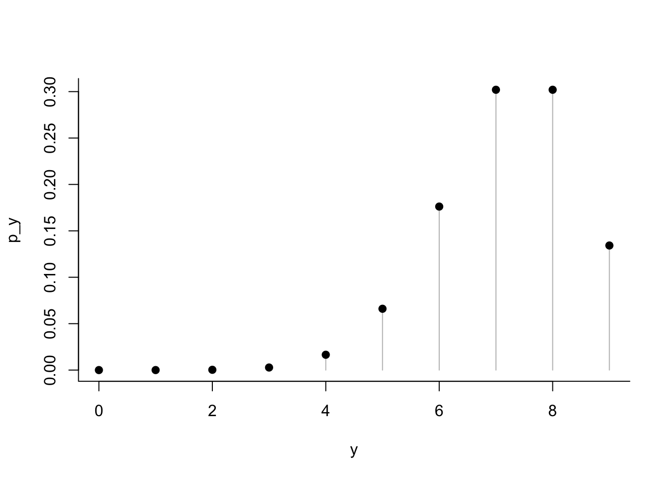
It is easy to check that this is a probability distribution: the values of p_y are positive and sum to 1.
sum(p_y)## [1] 1The sought probability in the example is \(P(Y=6) ≈ 0.1761\). (Be careful: this is the 7th item in the vector of probabilities because zero is the first value.)
11.2 Analytics in R: Defects in Semiconductors
The Poisson distribution in this example is concentrated on small integers.
x   <- 0:6
p_x <- dpois(x, lambda=314/400)cbind(x,p_x) # show a table with the probabilites## x p_x
## [1,] 0 0.4561197018
## [2,] 1 0.3580539659
## [3,] 2 0.1405361816
## [4,] 3 0.0367736342
## [5,] 4 0.0072168257
## [6,] 5 0.0011330416
## [7,] 6 0.0001482396plot(x, p_x, type='h', col='gray', bty='l', xlab="x", ylab="p(x)")
points(x,p_x, pch=19)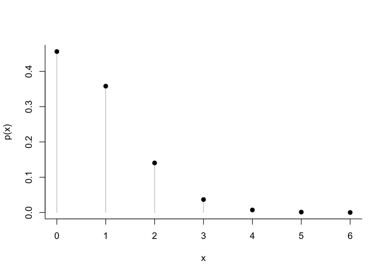
Notice that the Poisson probabilities in this table sum to a little less than 1. That’s because every Poisson distribution puts some probability on values all the way out to infinity.
sum(p_x)## [1] 0.9999816How much probability is left out, computed directly? Use ppois to find out.
1 - ppois(6, lambda=314/400) # 1 - P(X <= 6) = P(X > 6)## [1] 1.840955e-05