20 Curved Patterns

Plots remain front and center in this chapter. Regression models linear patterns, but many nonlinear patterns can be converted into linear patterns through a transformation of the data. Key functions in this chapter are:

plot graphs data on log scales when the option log is set coefficients extracts the estimated intercept and slope from a regression seq generates a sequence of values with arbitrary spacing lines adds a collection of line segments to a plot

20.1 Analytics in R: Optimal Pricing

Read the data into a data frame. These are sales of orange juice at 50 locations and at varying prices.

OJ <- read.csv("Data/20_4m_juice.csv")
dim(OJ)

## [1] 50  2

Each row gives the number of units sold at the indicated price.

head(OJ)

##   Sales Price
## 1    43   1.5
## 2    12   3.9
## 3    15   3.8
## 4    27   1.9
## 5     8   4.2
## 6    12   4.1

The association is not linear. Sales fall rapidly as the price moves away from about $1 and then decline at a slower rate from $2.50 and higher.

plot(Sales ~ Price, data=OJ)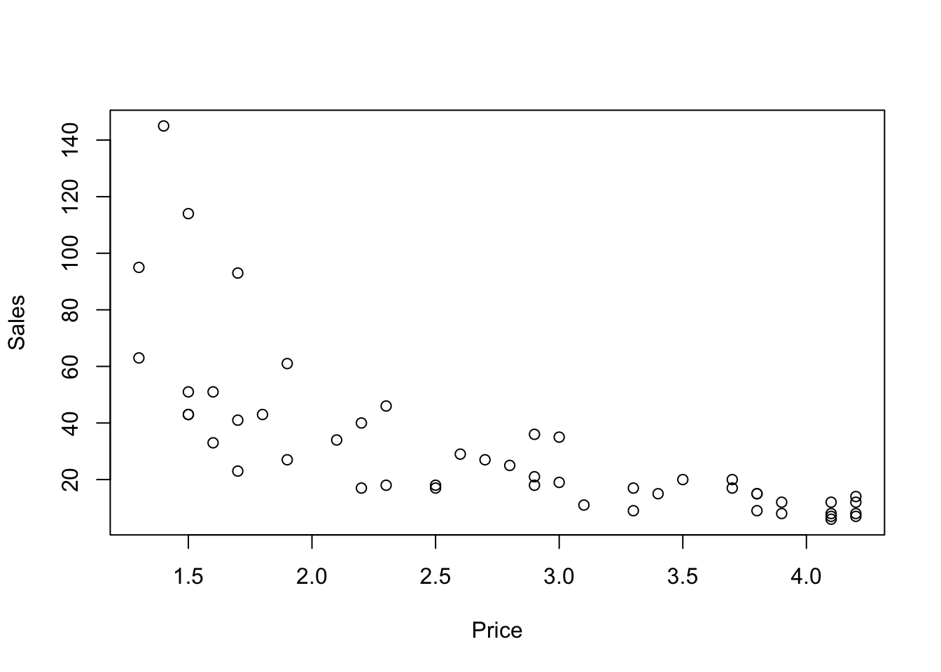

The association appears linear when expressed on a log-log scale. plot graphs the data with log scales labeled in the original units when the axes are identified in the log option. You can use log scales on both axes (as in this example), or just one.

plot(Sales ~ Price, data=OJ, log='xy')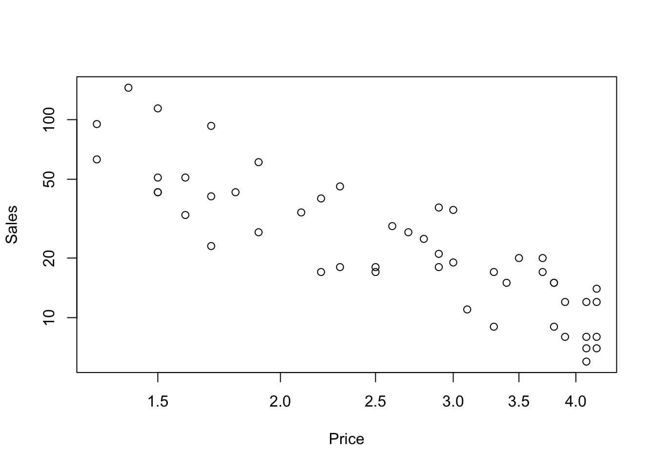

Notice that the previous plot is equivalent to a plot with both variables transformed to a log scale.

plot(log(Sales) ~ log(Price), data=OJ)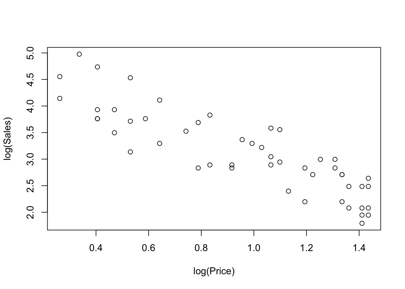

The points in the scatterplot are identical, but the labeling on the axes differs. I prefer the first version with more interpretable axes; you have to understand log scales to know what 0.8 on a log scale might mean. The plot labeled with actual sales and prices is much easier to interpret, but that sort of plot will not always be available.

A least squares regression captures the log-linear pattern nicely. Notice that the regression model needs to be on log scales as well. In order to add the line to the plot easily, I need to use the less attractive log scales.

plot(log(Sales) ~ log(Price), data=OJ)           # graph on log scales
regr <- lm(log(Sales) ~ log(Price), data=OJ)
abline(regr, col='red')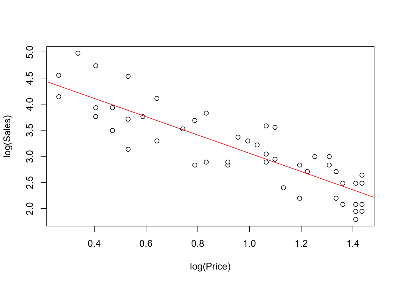

Print the regression object to see the estimated slope and intercept. The estimated slope is the estimated elasticity of sales with respect to price.

regr

## 
## Call:
## lm(formula = log(Sales) ~ log(Price), data = OJ)
## 
## Coefficients:
## (Intercept)   log(Price)  
##       4.812       -1.752

If you want to see more digits of these estimates, use the function coefficients to get a vector that has two elements, the estimated intercept and slope.

coefficients(regr)

## (Intercept)  log(Price) 
##    4.811646   -1.752383

It is a bit more tedious to show the curve associated with this fitted equation on the original scales, but usually worth it. abline draws a line for us, but there’s not a comparable function called curve. We need to compute the fitted values from the model on a grid of closely spaced values, then connect these points with lines in the a plot. This plot emphasizes the changing impact of prices changes on sales; the prior plots emphasize the constant elasticity.

plot(Sales ~ Price, data=OJ)       # plot on original units

x  <- seq(1,5,length.out=100)      # grid that extends over the range of x-axis

ab  <- coefficients(regr)          # intercept and slope, to full precision
fit <- exp(ab[1] + ab[2]*log(x))

lines(x, fit, col='red')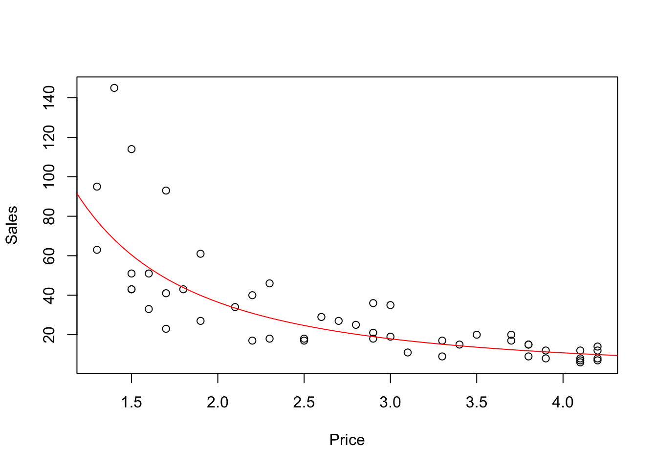

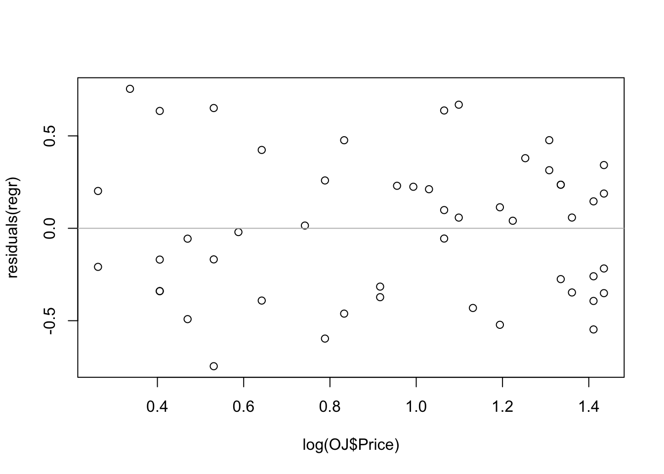
The residuals from the log-log regression do not show any evident pattern (albeit they seem a bit more concentrated on the right-hand side of the figure).

plot(log(OJ$Price), residuals(regr))
abline(h=0, col='gray')