21 The Simple Regression Model
The main difference in this chapter regarding the use of R from that in the prior 2 chapters is that we will look deeper into the regression object produced by lm. The result of summarizing the regression is a list with a number of useful components. Printing the summary shows a thorough summary of the fitted model that includes several test statistics. Key functions in this chapter are
lmfits a least squares regression and returns an object with further detailssummaryproduces a regression object with additional useful componentspredictproduces the exact prediction intervals for a regression model
21.1 Analytics in R: Locating a Franchise Outlet
Read the data into a data frame. The data frame has 80 observations of two variables.
Franchise <- read.csv("Data/21_4m_franchise.csv")
dim(Franchise)
## [1] 80 2Each row of the data frame describes the amount of gasoline sales (in thousands of gallons) and the traffic volume, also in thousands.
head(Franchise)## Sales Traffic
## 1 6.64 33.6
## 2 7.76 37.2
## 3 9.56 48.0
## 4 6.29 33.7
## 5 10.18 45.1
## 6 4.68 28.8A scatterplot of sales on traffic volume shows that the two variables are linearly associated. The association is moderately strong.
plot(Sales ~ Traffic, data=Franchise)

regr <- lm(Sales ~ Traffic, data=Franchise)
abline(regr, col='red')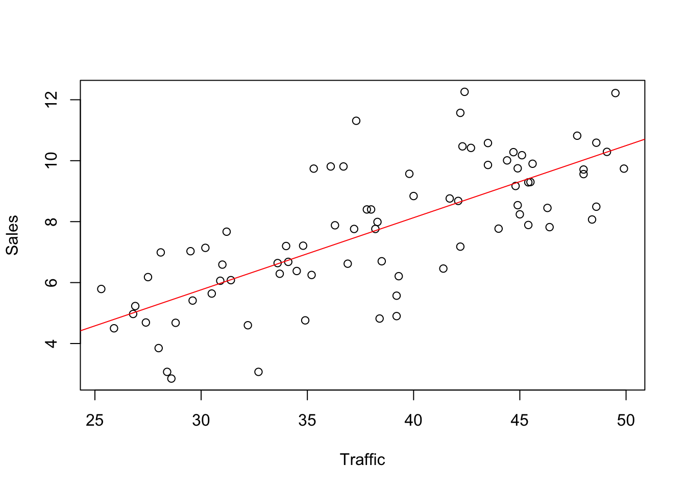
The summary of a regression holds a named list of properties of the regression,
sRegr <- summary(regr)
names(sRegr)
## [1] "call" "terms" "residuals" "coefficients"
## [5] "aliased" "sigma" "df" "r.squared"
## [9] "adj.r.squared" "fstatistic" "cov.unscaled"Printing the summary shows a table of the least squares estimates and the overall fit of the regression.
sRegr##
## Call:
## lm(formula = Sales ~ Traffic, data = Franchise)
##
## Residuals:
## Min 1Q Median 3Q Max
## -3.3329 -0.8684 0.0144 0.8478 3.8181
##
## Coefficients:
## Estimate Std. Error t value Pr(>|t|)
## (Intercept) -1.33810 0.94584 -1.415 0.161
## Traffic 0.23673 0.02431 9.736 4.06e-15 ***
## ---
## Signif. codes: 0 '***' 0.001 '**' 0.01 '*' 0.05 '.' 0.1 ' ' 1
##
## Residual standard error: 1.505 on 78 degrees of freedom
## Multiple R-squared: 0.5486, Adjusted R-squared: 0.5428
## F-statistic: 94.79 on 1 and 78 DF, p-value: 4.06e-15Before relying on the summary statistics for inference, check that the residuals do not show an evident pattern.
plot(Franchise$Traffic, residuals(regr))
abline(h=0, col='gray')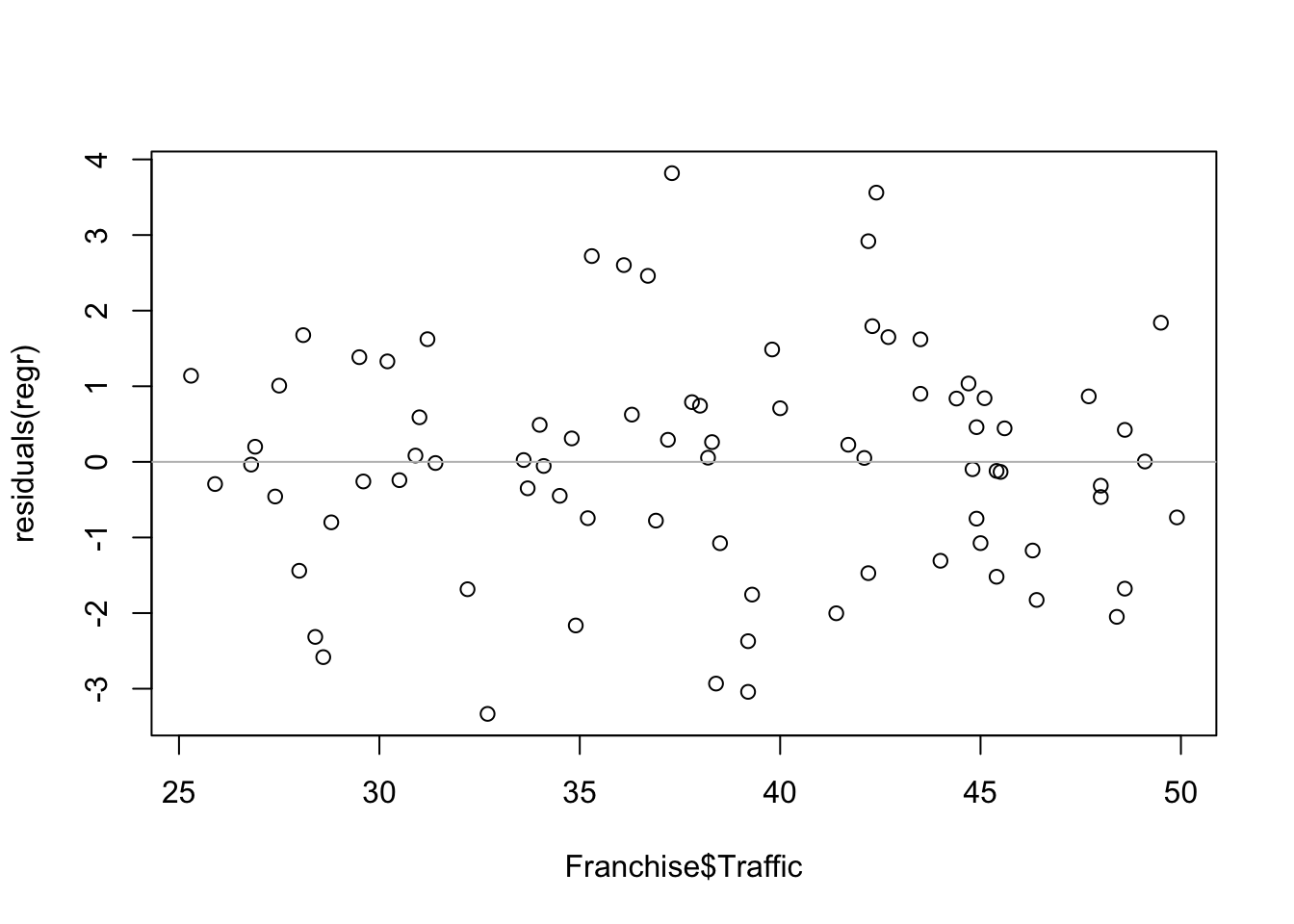
In addition check that the distribution of the residuals appears nearly normal. To get the bands, use the version of the normal quantile plot from the car package (see Chapter 12).
require(car)
qqPlot(residuals(regr))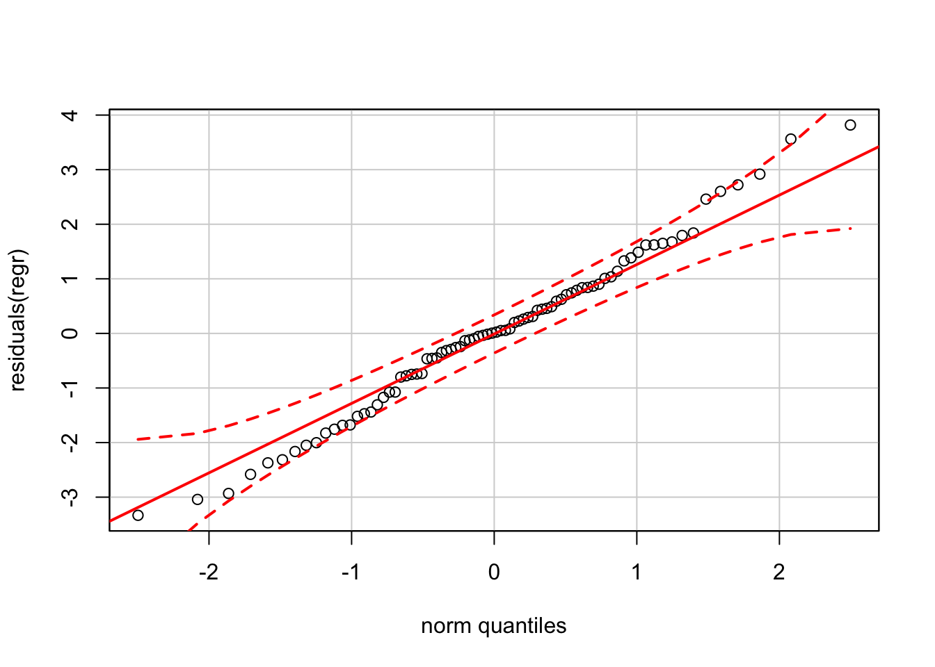
At the extremes, the residuals seem to be a bit “fat-tailed”, more extreme that what normality would expect. The deviation is slight, but worth noting. (The version of the normal QQ plot from car produces tighter bands than the reference software (JMP) software that was used to generate the figures that appear in the textbook.)
21.2 Analytics in R: Climate Change
These data give the global CO2 level and temperature recorded annually over 58 years, dating back to 1958.
Climate <- read.csv("Data/21_4m_climate.csv")
dim(Climate)
## [1] 58 3head(Climate)## Year CO2 Temperature
## 1 1958 315.2830 0.06
## 2 1959 315.9742 0.03
## 3 1960 316.9075 -0.03
## 4 1961 317.6367 0.05
## 5 1962 318.4500 0.02
## 6 1963 318.9942 0.06The time patterns are important to appreciate. The growth in CO2 levels in the atmosphere has been steady, with a gradually increasing slope.
plot(CO2 ~ Year, data=Climate)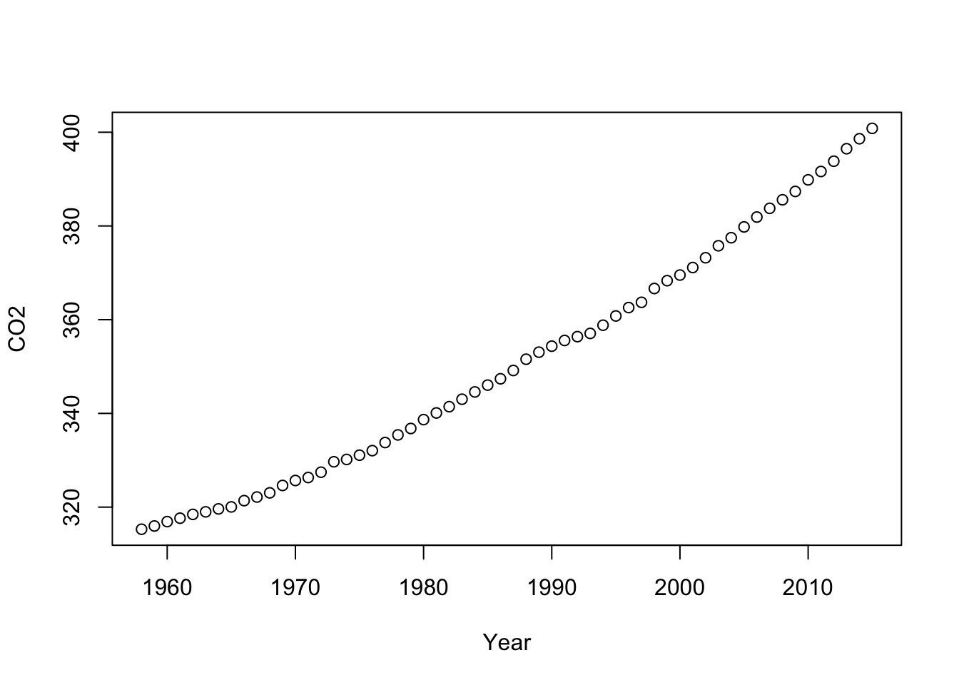
Temperature has also increased, but with much more variation around the upward trend.
plot(Temperature ~ Year, data=Climate)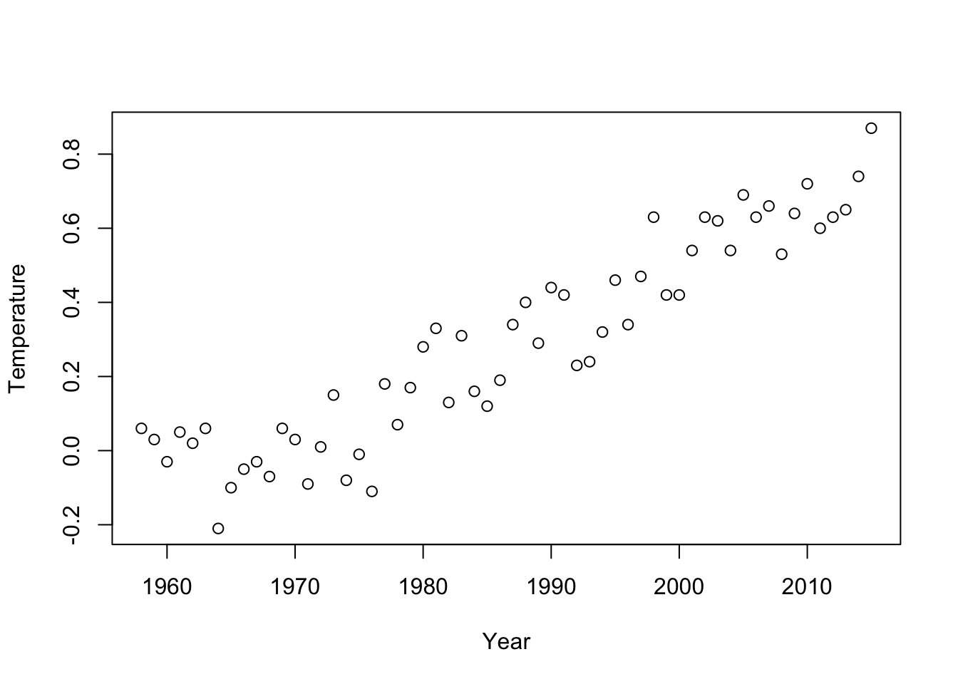
The association between CO2 and temperature is strong and linear.
plot(Temperature ~ CO2, data=Climate)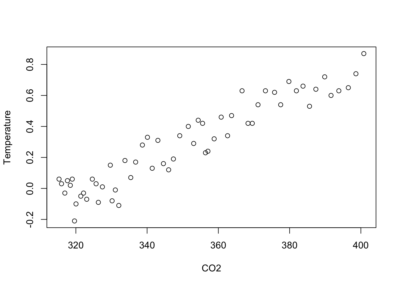
We can add the fitted regression to this plot and the region defined by the 95% prediction intervals from the regression. For getting the prediction intervals, first choose a grid of points along the CO2 axis; this grid should extend far enough to span the range of the x-axis in the scatterplot.
Next use the function predict to obtain the prediction intervals from the regression at the points on this grid. predict requires a data frame to indicate the values of the explanatory variable. A variable in the data frame given to predict must have the same name as the explanatory variable in the regression.
plot(Temperature ~ CO2, data=Climate)

regr <- lm(Temperature ~ CO2, data=Climate)
abline(regr, col='red')

grid <- data.frame(CO2 = seq(300,450, length.out=50))   # 50 makes the grid fine enough

predint <- predict(regr, newdata=grid, interval='prediction')

lines(grid$CO2, predint[,"lwr"], lty=2)   # lower limit of prediction interval
lines(grid$CO2, predint[,"upr"], lty=2)   # upper limit of prediction interval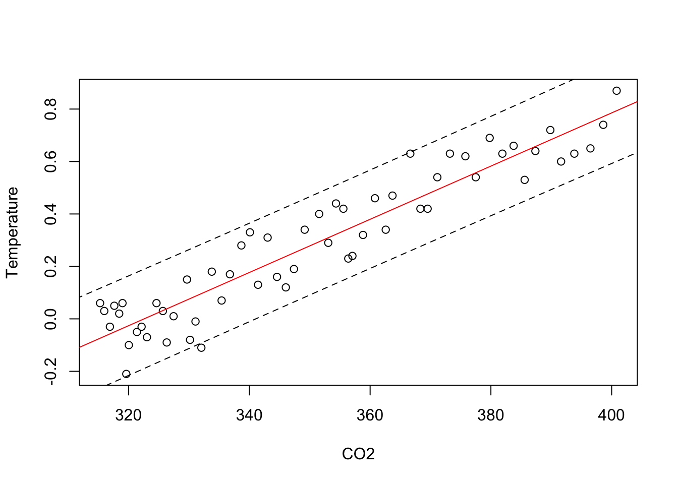
Here are the details of the regression.
summary(regr) ##
## Call:
## lm(formula = Temperature ~ CO2, data = Climate)
##
## Residuals:
## Min 1Q Median 3Q Max
## -0.206300 -0.065396 -0.009465 0.077352 0.182671
##
## Coefficients:
## Estimate Std. Error t value Pr(>|t|)
## (Intercept) -3.2725929 0.1685211 -19.42 <2e-16 ***
## CO2 0.0101456 0.0004788 21.19 <2e-16 ***
## ---
## Signif. codes: 0 '***' 0.001 '**' 0.01 '*' 0.05 '.' 0.1 ' ' 1
##
## Residual standard error: 0.09277 on 56 degrees of freedom
## Multiple R-squared: 0.8891, Adjusted R-squared: 0.8871
## F-statistic: 448.9 on 1 and 56 DF, p-value: < 2.2e-16The sequence plot of residuals does not show an evident pattern.
plot(Climate$Year, residuals(regr), type='l')
abline(h=0, col='gray')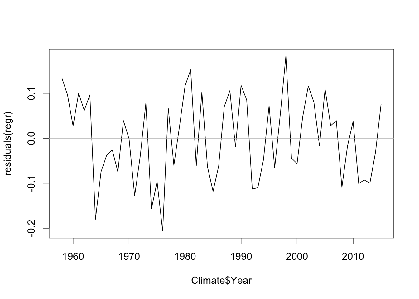
The other diagnostic plots also seem okay. There’s no strong pattern in the plot of residuals on the explanatory variable, but something looks to be happening: might there be a trend that we’ve missed.
plot(Climate$CO2, residuals(regr))
abline(h=0, col='gray')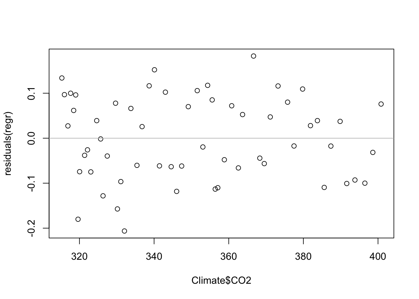
The residuals also appear nearly normal.
require(car)
qqPlot(residuals(regr))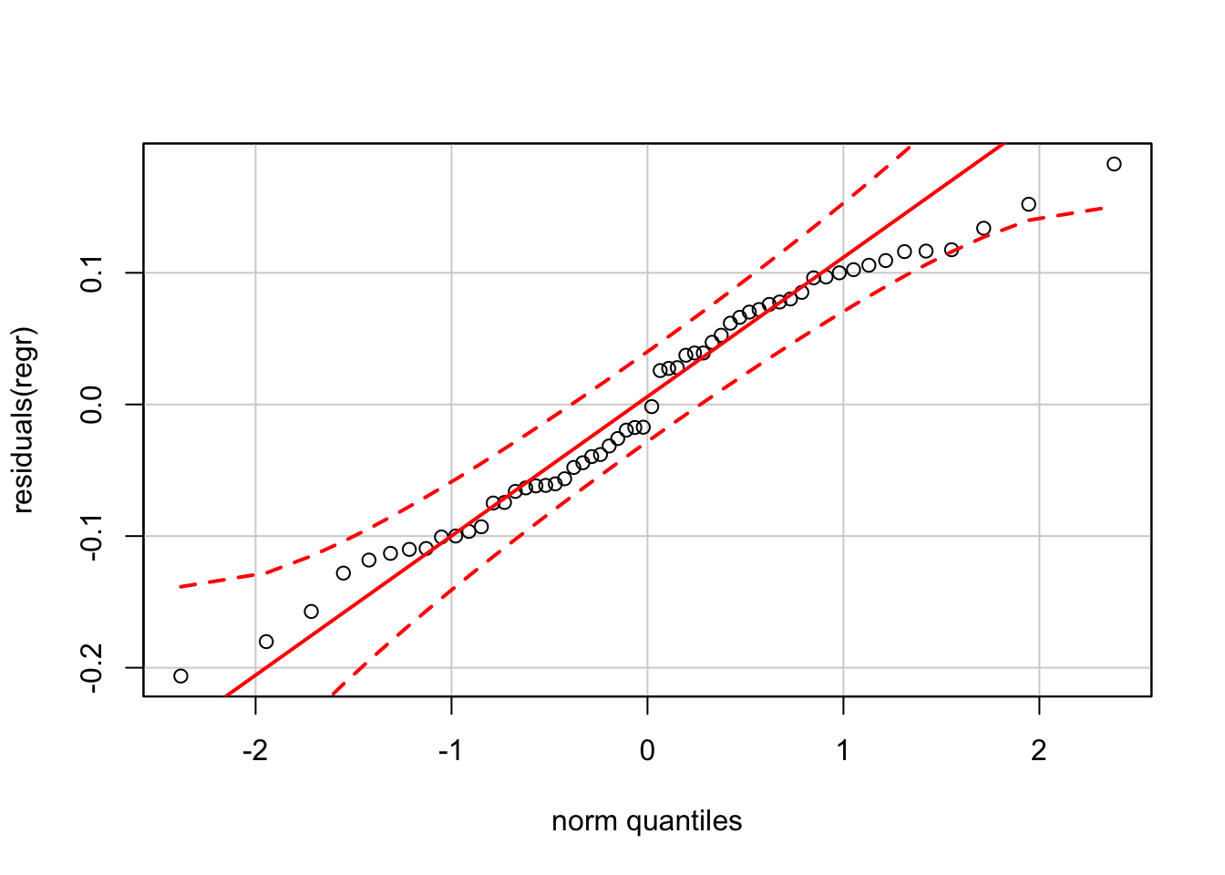
To get the exact prediction interval at a single point requires the same approach used for the grid of points added to the plot. Namely, construct a data frame with a variable named as the explanatory variable in the regression (here, “CO2”), and then use this data frame as the newdata argument to the function predict.
new <- data.frame(CO2 = c(380, 425))

predict(regr, newdata=new, interval='prediction')
## fit lwr upr
## 1 0.5827394 0.3932505 0.7722283
## 2 1.0392919 0.8388671 1.2397167You can check that the small differences between the values shown here for the prediction interval and those in the textbook presentation are due to rounding.