24 Building Regression Models
The examples in this chapter use tools introduced in prior chapters on regression. Some new functions considered here include
rownamesassigns names to the rows in a data filecoefficientsextracts coefficient estimates from a modelidentify“interactively” uses the cursor to label points in a scatterplot
24.1 Analytics in R: Market Segmentation
The cases in this data set record the characteristics and reactions of 75 consumers of varying ages and incomes to a new smartphone design.
Segment <- read.csv("Data/24_4m_segmentation.csv")
dim (Segment)
## [1] 75 4head(Segment)## Rating Age Income Income_Group
## 1 4.4 56.8 127.8
## 2 3.4 52.0 118.7 Med
## 3 3.5 29.1 72.7 Low
## 4 7.4 67.4 164.8 High
## 5 7.9 70.7 185.7 High
## 6 4.4 47.1 114.4 MedThe scatterplot matrix with added correlations shows the extensive collinearity that complicates this example. The correlation between the two explanatory variables is 0.82.
source("functions.R")
pairs(Segment[,1:3], lower.panel=panel.cor)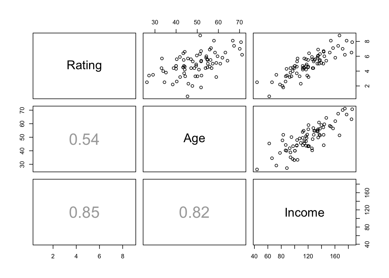
The multiple regression of Rating on Age and Income follows. The multiple regression is perhaps surprising because the partial slope of the variable Age is negative (and significantly so) whereas the correlation between Age and Rating is positive. (Given some thought, however, it is the positive marginal correlation between Age and Rating that is perhaps the more surprising correlation.)
regr <- lm(Rating ~ Age + Income, data=Segment)
summary(regr)
##
## Call:
## lm(formula = Rating ~ Age + Income, data = Segment)
##
## Residuals:
## Min 1Q Median 3Q Max
## -2.1100 -0.4259 0.1573 0.4359 1.5550
##
## Coefficients:
## Estimate Std. Error t value Pr(>|t|)
## (Intercept) 0.513864 0.412504 1.246 0.217
## Age -0.079784 0.014449 -5.522 5.03e-07 ***
## Income 0.069205 0.004981 13.894 < 2e-16 ***
## ---
## Signif. codes: 0 '***' 0.001 '**' 0.01 '*' 0.05 '.' 0.1 ' ' 1
##
## Residual standard error: 0.707 on 72 degrees of freedom
## Multiple R-squared: 0.8075, Adjusted R-squared: 0.8022
## F-statistic: 151 on 2 and 72 DF, p-value: < 2.2e-16The plot of residuals on fitted values shows no problem.
plot(residuals(regr) ~ fitted.values(regr))
abline(h=0, col='gray')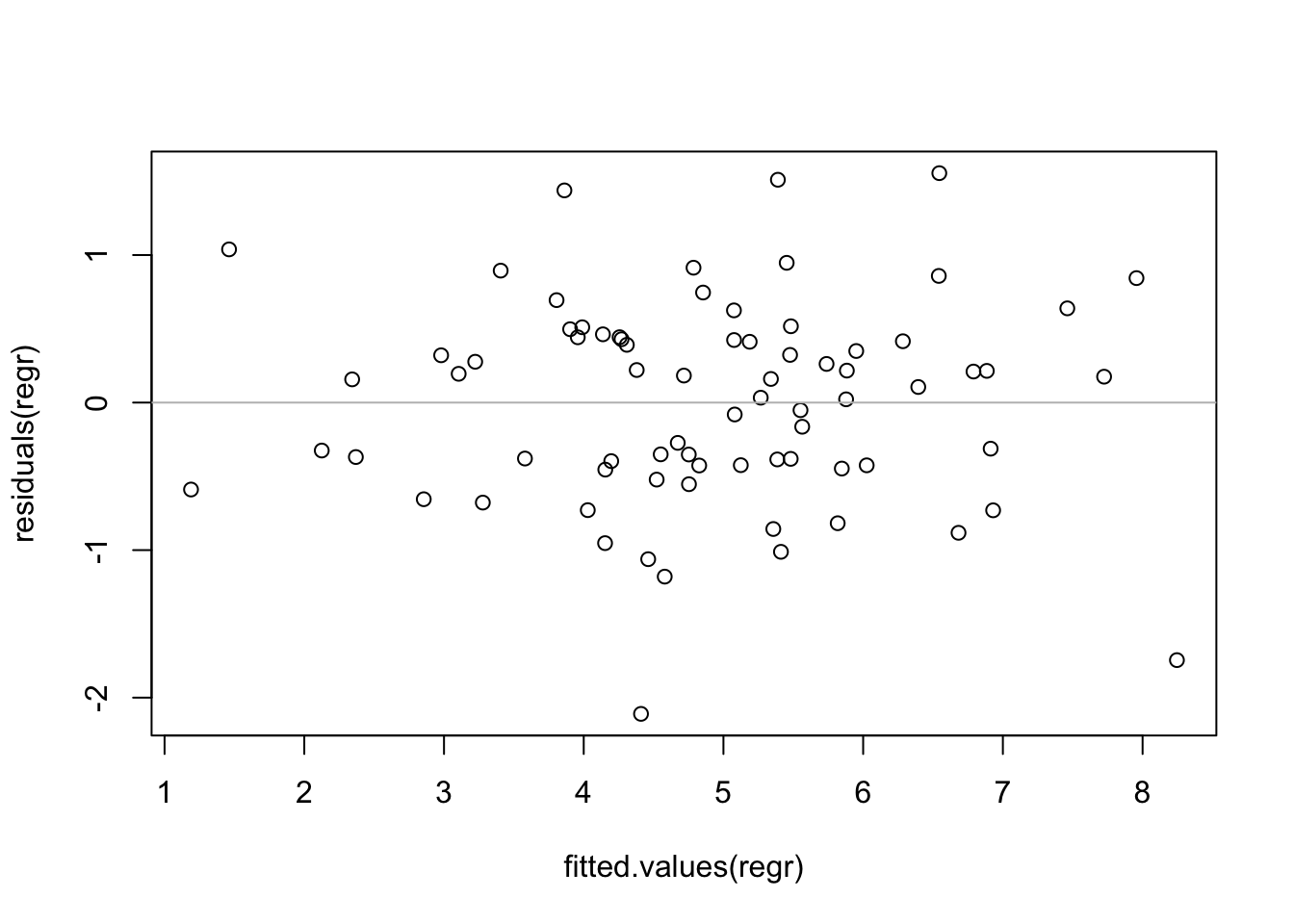
The residuals are also “nearly normal”, though there is an odd “kink” produced by several widely spaced residuals near 0. Residuals near 0 are typically more tightly clustered than those farther from 0.
require(car)
qqPlot(residuals(regr))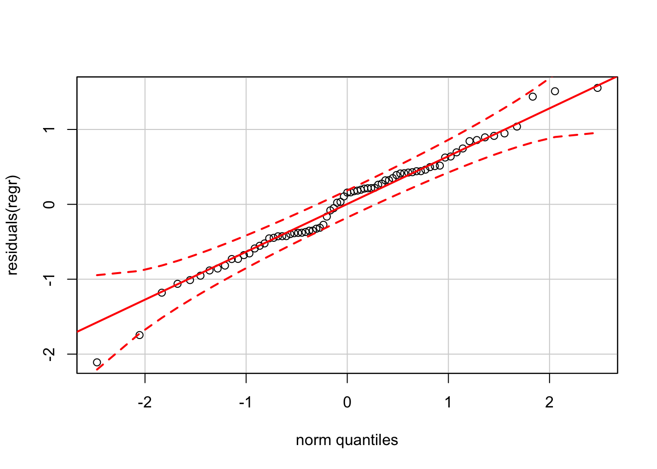
24.2 Analytics in R: Retail Profits
These data record the profitability of drug stores located in 111 communities around the US. Other variables in the data set describe economic and demographic characteristics of the communities.
Retail <- read.csv("Data/24_4m_retail_profit.csv")
dim(Retail)
## [1] 111 8head(Retail)## Location Profit Income Disp_Income Birth_Rate
## 1 Albany-Schenectady-Troy,NY 199780 28719 22701 13.1
## 2 Albuquerque,NM 165530 25835 19890 15.8
## 3 Altoona,PA 208670 22675 18051 11.6
## 4 Anchorage,AK 166890 33501 27031 18.5
## 5 Appleton-Oshkosh-Neenah,WI 209190 27107 21182 13.6
## 6 Athens,GA 162600 23304 18148 12.9
## Soc_Security CV_Death Pct65
## 1 177.7 429.9 14.6
## 2 143.8 222.9 10.7
## 3 179.8 561.5 17.6
## 4 62.5 99.8 4.7
## 5 152.6 319.4 12.0
## 6 125.4 254.6 9.4Rather than leave the location as a variable in the data frame, it will be more convenient in this example to use these names to label the rows instead. We won’t lose the information, but R won’t treat these labels as a variable.
rownames(Retail) <- Retail$Location    # assign row labels
Retail$Location <- NULL                # remove the original column
Now the rows of the Retail data frame are labeled by the location. Notice that the last row of the data table does not include the profit. We want a prediction for this location.
Retail[110:111,]## Profit Income Disp_Income Birth_Rate Soc_Security
## Youngstown-Warren,OH 211620 25981 19155 12.8 212.3
## KansasCity,MO-KS NA 28774 22642 14.4 148.8
## CV_Death Pct65
## Youngstown-Warren,OH 477.9 16.2
## KansasCity,MO-KS 338.5 11.4We will need to exclude this last row from some calculations. For example, R returns a missing value (denoted by NA) for the average profit.
mean(Retail$Profit)## [1] NAMissing values are “contagious” in R in the sense that these contaminate calculations in which they are included. For example, NA + 7 results in NA. That makes sense when you think about it. If you add an unknown quantity to a known quantity, the sum too is unknown. plot simply omits missing values, but functions like sum don’t know the sum if this last row is included, so they simply return NA.
The scatterplot matrix shows some obvious sources of collinearity. For example, locations with older residents have both higher payments from Social Security as well as more cardio-vascular diseases. (I omit columns to get a figure like that in the textbook.)
pairs(Retail[,c(1,4:7)], lower.panel=panel.cor)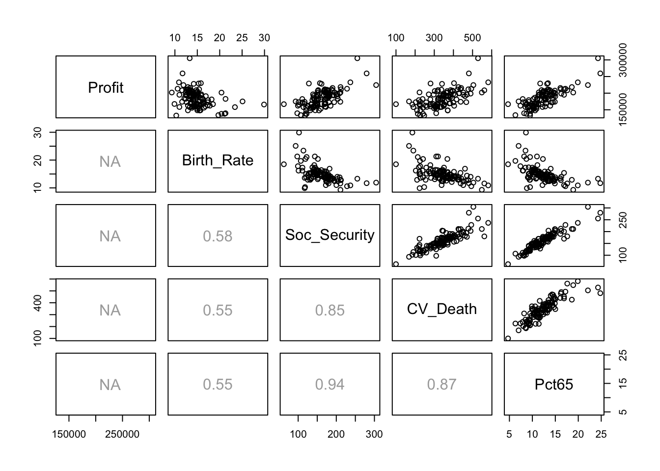
Notice that all of the correlations involving Profit are shown as missing (NA). That’s because the last observation does not include a value for the profit. It’s easy to “fix” this problem by excluding the last row by using a negative index.
pairs(Retail[-111,c(1,4:7)], lower.panel=panel.cor)
Here is the summary of the multiple regression that includes all six explanatory variables. This version of the formula for the regression uses a period rather than listing the explanatory variables. A single period on the right-hand side of a formula tells R to use all of the variables in the data frame as explanatory variables except for the response. (Note: this specification would not work had we left Location as a variable in the data frame. R would have tried to use it as a factor in the model.)
regr <- lm(Profit ~ ., data=Retail)
summary(regr)
##
## Call:
## lm(formula = Profit ~ ., data = Retail)
##
## Residuals:
## Min 1Q Median 3Q Max
## -31588 -10096 646 9067 30454
##
## Coefficients:
## Estimate Std. Error t value Pr(>|t|)
## (Intercept) 13161.3422 19111.3903 0.689 0.492582
## Income 0.5986 0.5887 1.017 0.311598
## Disp_Income 2.5350 0.7318 3.464 0.000776 ***
## Birth_Rate 1703.8657 563.6726 3.023 0.003161 **
## Soc_Security -47.5162 110.2129 -0.431 0.667274
## CV_Death -22.6821 31.4642 -0.721 0.472613
## Pct65 7713.8505 1316.2100 5.861 5.59e-08 ***
## ---
## Signif. codes: 0 '***' 0.001 '**' 0.01 '*' 0.05 '.' 0.1 ' ' 1
##
## Residual standard error: 13550 on 103 degrees of freedom
## (1 observation deleted due to missingness)
## Multiple R-squared: 0.7558, Adjusted R-squared: 0.7415
## F-statistic: 53.12 on 6 and 103 DF, p-value: < 2.2e-16The car package includes a function that computes the variance inflation factors.
require(car)
vif(regr)
## Income Disp_Income Birth_Rate Soc_Security CV_Death
## 2.953242 3.304986 1.699514 10.038173 4.710607
## Pct65
## 11.385537Because we assigned names to the rows, these names will be used when R draws the default diagnostic plots for this regression.
save <- par(mfrow=c(2,2))
plot(regr)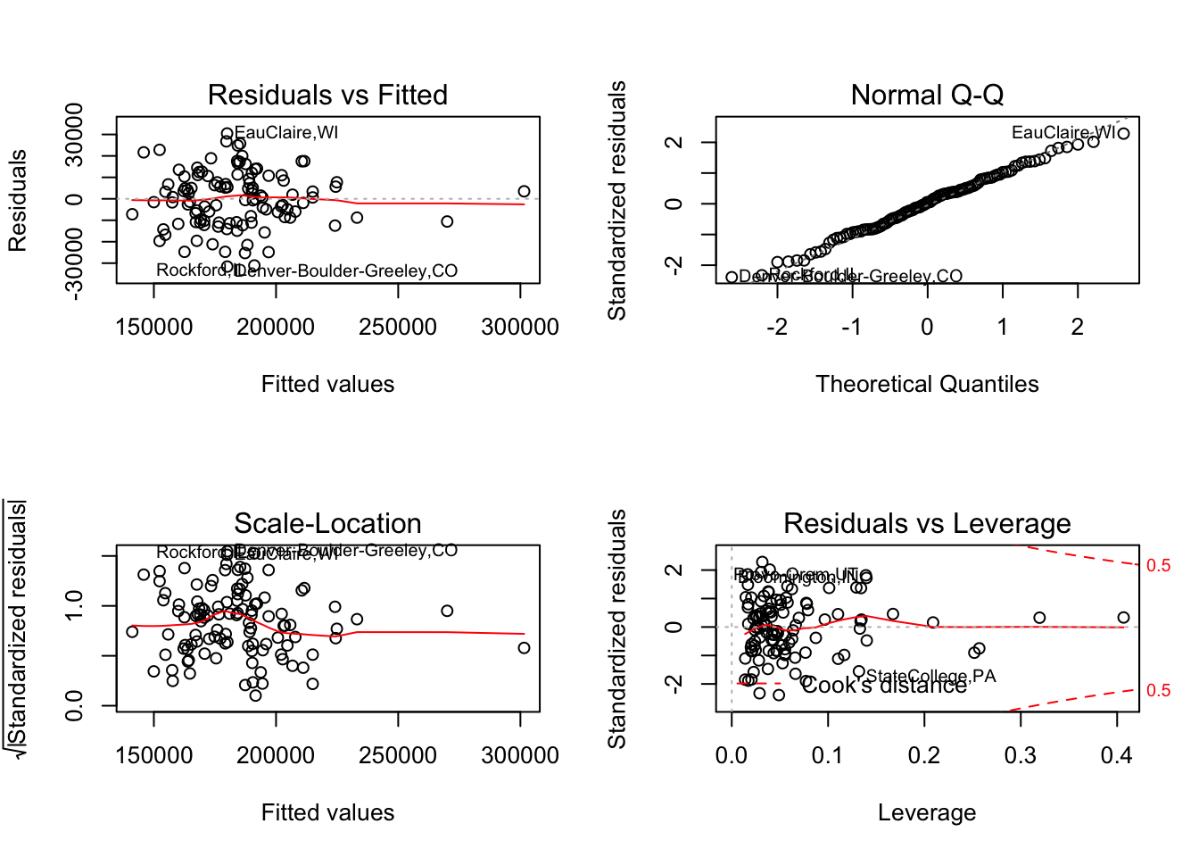
par(save)Which are the locations with the largest fitted values? We can use identify to figure that out. identify shows a scatterplot and allows you to click on points with the cursor. Type escape when you are done, and the row names for these points will appear. (You need to run this command from the console window if you are running these examples in R-Studio.)
plot(fitted.values(regr), residuals(regr))
identify(fitted.values(regr), residuals(regr), labels=rownames(Retail)[-111])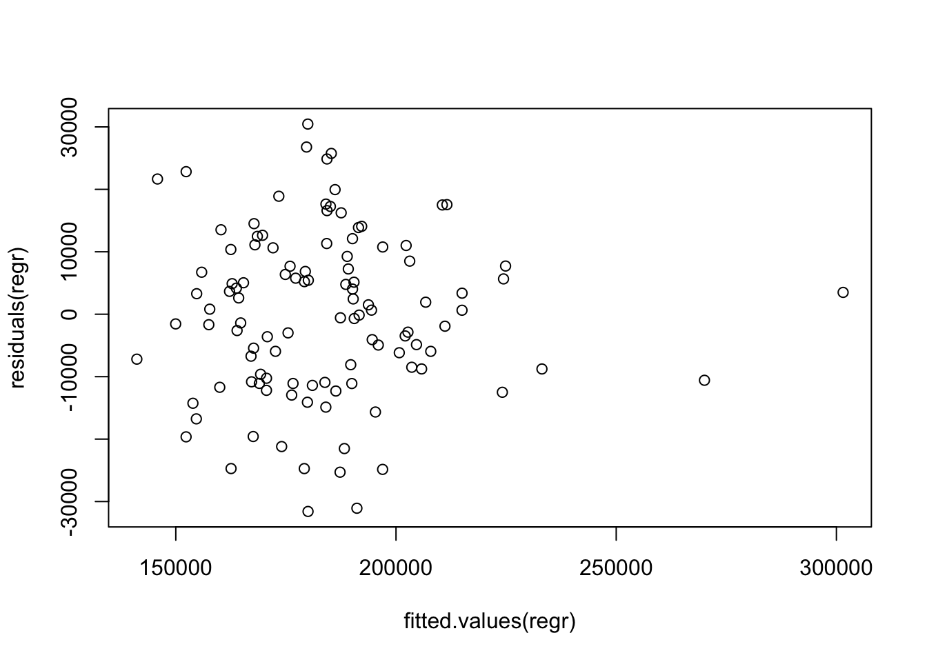
## integer(0)The result of identify is a vector of the indices in the source data of the points that you click on. In this case, I picked the two locations in Florida that are popular retirement destinations.
rownames(Retail)[c(40,108)]## [1] "FortMyers-CapeCoral,FL" "WestPalmBeach-BocaRaton,FL"Several variables in the regression are not statistically significant and can be removed to obtain a more parsimonious model that explains about the same amount of variation. (The adjusted \(R^2\) statistic is actually higher.) For use later, save the regression model in an object with a different name for the sake of comparing the predictions.
regr_2<- lm(Profit ~ Disp_Income + Birth_Rate + Pct65, data=Retail)
summary(regr_2)
##
## Call:
## lm(formula = Profit ~ Disp_Income + Birth_Rate + Pct65, data = Retail)
##
## Residuals:
## Min 1Q Median 3Q Max
## -30228.3 -9290.0 412.7 9428.1 30625.9
##
## Coefficients:
## Estimate Std. Error t value Pr(>|t|)
## (Intercept) 1.004e+04 1.534e+04 0.655 0.514147
## Disp_Income 3.239e+00 4.137e-01 7.828 3.98e-12 ***
## Birth_Rate 1.874e+03 5.265e+02 3.559 0.000558 ***
## Pct65 6.619e+03 4.655e+02 14.219 < 2e-16 ***
## ---
## Signif. codes: 0 '***' 0.001 '**' 0.01 '*' 0.05 '.' 0.1 ' ' 1
##
## Residual standard error: 13460 on 106 degrees of freedom
## (1 observation deleted due to missingness)
## Multiple R-squared: 0.7521, Adjusted R-squared: 0.745
## F-statistic: 107.2 on 3 and 106 DF, p-value: < 2.2e-16R presents the coefficients in this output in “scientific notation” with just 4 digits shown. To see the estimates and standard errors, use the function coefficients. coefficients applied to the regression object constructed by lm returns a vector with just estimated values. If applied to a summary of the regression, coefficients returns a matrix of values that includes estimates, standard errors, t-statistics, and p-values.
coefficients(summary(regr_2))## Estimate Std. Error t value Pr(>|t|)
## (Intercept) 10044.608543 1.534479e+04 0.654594 5.141471e-01
## Disp_Income 3.238622 4.137409e-01 7.827658 3.975462e-12
## Birth_Rate 1874.045436 5.265008e+02 3.559435 5.577280e-04
## Pct65 6619.207492 4.655340e+02 14.218526 2.590007e-26The final task in this case is to predict sales at the location described in row 111 that has the missing value for the profits (Kansas City). The predict function works in for a multiple regression in exactly the same way as in simple regression. Here is the predicted value and 95% prediction interval from the initial model with all of the explanatory variables.
predict(regr, newdata=Retail[111,], interval='prediction')## fit lwr upr
## KansasCity,MO-KS 185509.2 158366.8 212651.6The reduced model with just three explanatory variables produces a very similar prediction and interval.
predict(regr_2, newdata=Retail[111,], interval='prediction')## fit lwr upr
## KansasCity,MO-KS 185818.7 158901.9 212735.6