17 Comparison
As in previous chapters in this part of the book, we again use R in this chapter as a powerful calculator. You can take a different approach, however. R includes a function that does most of the work, t.test, and avoids making that extra assumption of equal variances. The examples here illustrate that function as well as show how to do the other calculations from scratch, for practice. Functions or new uses of functions that are introduced in this chapter are few:
boxplotdraws side-by-side comparisons of groupst.testcomputes two-sample t-statistics, avoiding the assumption of equal variances
17.1 Analytics in R: A/B Testing
The underlying data are in a file that can be used to obtain a contingency table.
Test <- read.csv("Data/17_4m_abtesting.csv")
dim(Test)
## [1] 2495 3Each row summarizes the behavior of a visitor to the web site. The first column is the ID number of the visitor, and the other two columns give the page viewed and whether the visitor added the item to the shopping cart.
head(Test)## Visitor Page_Viewed Add_To_Cart
## 1 892360 B No
## 2 154666 A No
## 3 100035 A No
## 4 904653 B No
## 5 796311 B No
## 6 864892 B NoWe can get the proportions from the contingency table. CrossTable (in the package gmodels introduced in Chapter 5) provides a good summary.
require(gmodels)
CrossTable(Test$Add_To_Cart,Test$Page_Viewed,
           prop.t=FALSE, prop.r=FALSE, prop.chisq=FALSE)  # suppress extraneous terms
##
##
## Cell Contents
## |-------------------------|
## | N |
## | N / Col Total |
## |-------------------------|
##
##
## Total Observations in Table: 2495
##
##
## | Test$Page_Viewed
## Test$Add_To_Cart | A | B | Row Total |
## -----------------|-----------|-----------|-----------|
## No | 1192 | 1198 | 2390 |
## | 0.975 | 0.942 | |
## -----------------|-----------|-----------|-----------|
## Yes | 31 | 74 | 105 |
## | 0.025 | 0.058 | |
## -----------------|-----------|-----------|-----------|
## Column Total | 1223 | 1272 | 2495 |
## | 0.490 | 0.510 | |
## -----------------|-----------|-----------|-----------|
##
## Define the needed sample statistics so that we can use expressions like those in the textbook for the confidence interval.
n_a <- 1223
n_b <- 1272

p_a <- 31/n_a
p_b <- 74/n_b

zquan <- -qnorm(0.025)   # approximately 1.96
The expression for the standard error is on the long side, but shared for both endpoints of the confidence interval.
(p_b - p_a) + c(-zquan,zquan) * sqrt( p_a*(1-p_a)/n_a + p_b*(1-p_b)/n_b )## [1] 0.01723788 0.04841931The interval does not include 0 and so we reject \(H_0\) that the two pages are equally effective. Page B has the higher conversion rate.
17.2 Analytics in R: Comparing Two Diets
Start by reading in the data.
Diet <- read.csv("Data/17_4m_diet.csv")
dim(Diet)
## [1] 63 6The analysis concerns the amount of weight lost by the 63 participants after six months on the diet.
head(Diet)## Diet Initial_Weight Weight_6_Month Weight_12_Month Loss_6_Months
## 1 Atkins 310 292.7 286.1 17.3
## 2 Atkins 309 275.1 306.3 33.9
## 3 Atkins 257 217.7 263.3 39.3
## 4 Atkins 227 221.1 216.8 5.9
## 5 Atkins 231 204.5 211.8 26.5
## 6 Atkins 195 148.0 174.5 47.0
## Loss_12_Months
## 1 23.9
## 2 2.7
## 3 -6.3
## 4 10.2
## 5 19.2
## 6 20.5The function boxplot can draw boxplots side-by-side to compare data in two or more groups. We can use the formula notation introduced in Chapter 6 to define the variables in the plot. The variable to the left of the ~ defines the y-axis and the variable to the right of ~ defines the x-axis.
boxplot(Loss_6_Months ~ Diet, data=Diet)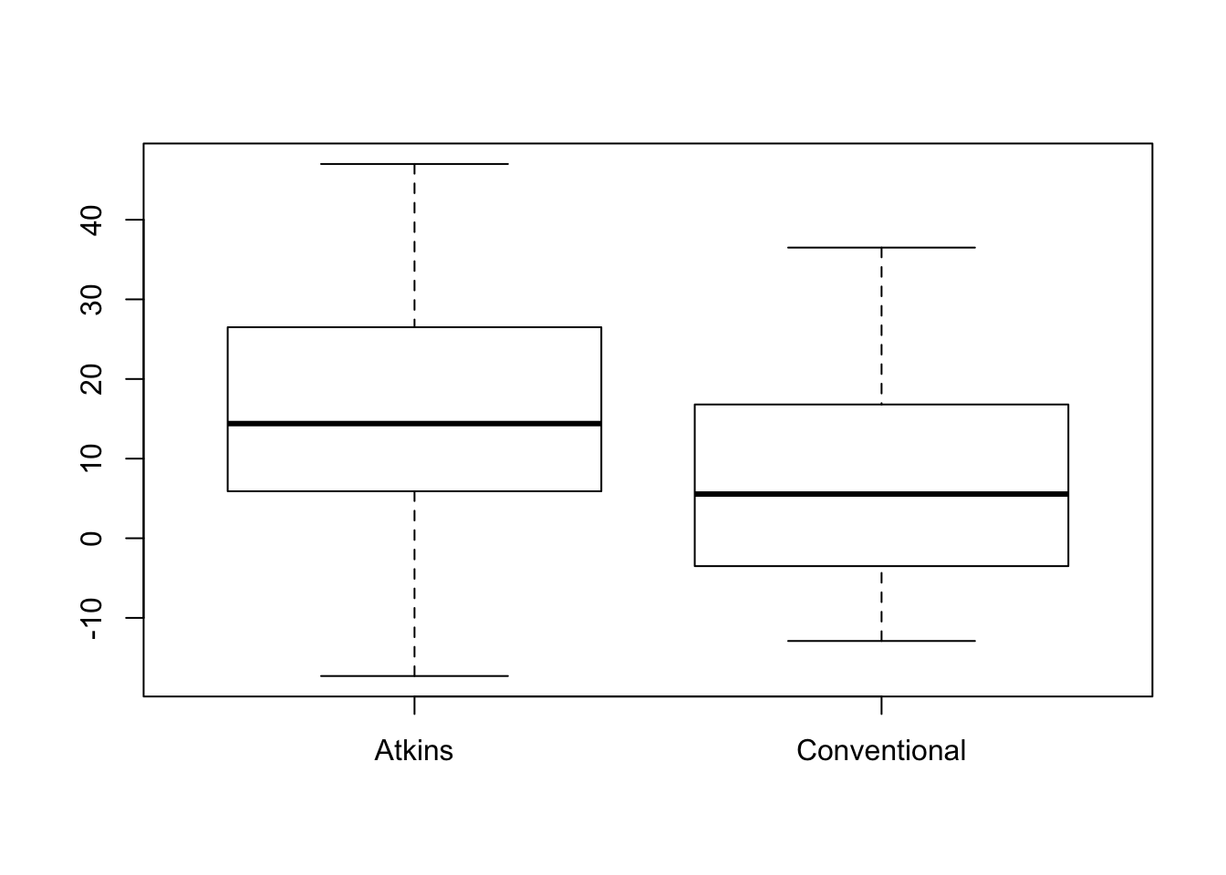
The boxplots appear reasonably symmetric, but these are small samples. We need to check the kurtosis of the two groups. Use tapply (illustrated in Chapter 14). The sample estimates of \(K_4\) are small enough so that we meet the sample size condition in both samples.
require(moments)
tapply(Diet$Loss_6_Months, Diet$Diet, kurtosis) - 3
## Atkins Conventional
## -0.09135406 -0.66857151Now compute the relevant summary statistics for each group using tapply again.
n    <- tapply(Diet$Loss_6_Months, Diet$Diet, length)
xbar <- tapply(Diet$Loss_6_Months, Diet$Diet, mean)
s    <- tapply(Diet$Loss_6_Months, Diet$Diet, sd)
For example, xbar is a two-element vector with the mean of each group.
xbar## Atkins Conventional
## 15.424242 7.006667These sample statistics determine the t-statistic. Don’t forget to subtract off the break-even value 5 from the difference between the means.
t_stat <- (xbar[1]-xbar[2] - 5)/sqrt(s[1]^2/n[1] + s[2]^2/n[2])
t_stat
## Atkins
## 1.014365Assuming equal variances in the two populations (see the discussion in the textbook), we can use pt to find the p-value.
1 - pt(t_stat, df=sum(n)-2)## Atkins
## 0.1572075To get the more sophisticated version of the t-statistic that does not require the data come from populations with equal variances, use the function t.test. You supply the data to this function as two separate vectors. In this case, use the values in the column Diet to identify observations in the “Atkins” and “Conventional” groups. The test statistic is the same, but the p-value is substantially larger.
group_a <- Diet$Loss_6_Months[Diet$Diet=="Atkins"]
group_c <- Diet$Loss_6_Months[Diet$Diet=="Conventional"]

t.test(group_a, group_c, mu=5)
##
## Welch Two Sample t-test
##
## data: group_a and group_c
## t = 1.0144, df = 60.826, p-value = 0.3144
## alternative hypothesis: true difference in means is not equal to 5
## 95 percent confidence interval:
## 1.68010 15.15505
## sample estimates:
## mean of x mean of y
## 15.424242 7.00666717.3 Analytics in R: Evaluating a Promotion
Start by reading the data file.
Promo <- read.csv("Data/17_4m_promo.csv")
dim(Promo)
## [1] 125 2Each row describes the awareness and number of mailings used by one of the 125 visited offices.
head(Promo)## Awareness Mailings
## 1 NO 15
## 2 NO 49
## 3 NO 42
## 4 NO 0
## 5 NO 26
## 6 NO 35The boxplots look similar and symmetric.
boxplot(Mailings ~ Awareness, data=Promo)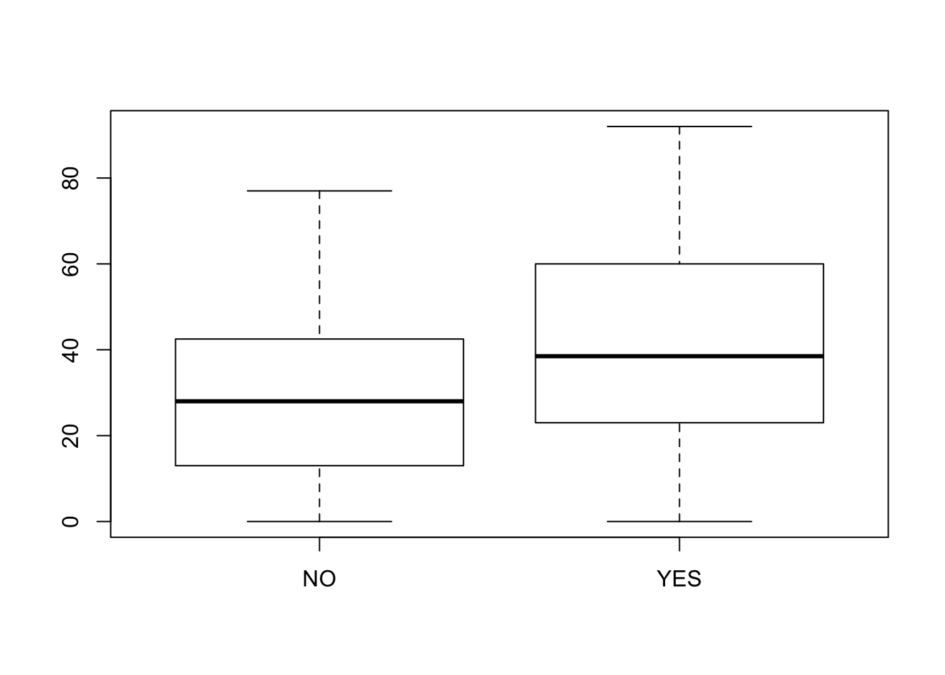
The estimated excess kurtosis in the two samples confirms that we have enough data to meet the sample size condition.
require(moments)
tapply(Promo$Mailings, Promo$Awareness, kurtosis) - 3
## NO YES
## -0.7326079 -0.9457113Use tapply as in the prior example to find the sample statistics for each group. Notice that the first element in each vector describes the “No” group (those that were not aware of the promotion prior to the visit).
n    <- tapply(Promo$Mailings, Promo$Awareness, length)
xbar <- tapply(Promo$Mailings, Promo$Awareness, mean)
s    <- tapply(Promo$Mailings, Promo$Awareness, sd)
We can compute the test statistic by almost copying the same formula used in the prior example.
t_stat <- (xbar[1]-xbar[2])/sqrt(s[1]^2/n[1] + s[2]^2/n[2])
t_stat
## NO
## -2.886651You can guess now that the confidence interval won’t include zero. Let’s check that. (Again, I am assuming variances match in the two populations to simplify finding the degrees of freedom for the t-quantile. The two intervals are very similar, particularly after rounding.)
The confidence interval for \(\mu_{yes}-\mu_{no}\) is then
t_quant <- -qt(0.025, df=sum(n)-2)

ci <- (xbar[2]-xbar[1]) + c(-t_quant, t_quant) * sqrt(s[1]^2/n[1] + s[2]^2/n[2])
ci
## [1] 3.867722 20.745611round(ci,1)## [1] 3.9 20.7To avoid the details, use the function t.test. You just have to collect the data for the two groups into separate samples. In this example, the results are slightly more significant than found using the just-illustrated procedure that assumes equal variances. (Be careful typing the names of the groups; R is case sensitive.)
group_y <- Promo$Mailings[Promo$Awareness=="YES"]
group_n <- Promo$Mailings[Promo$Awareness=="NO"]

t.test(group_y, group_n)
##
## Welch Two Sample t-test
##
## data: group_y and group_n
## t = 2.8867, df = 85.166, p-value = 0.004933
## alternative hypothesis: true difference in means is not equal to 0
## 95 percent confidence interval:
## 3.830319 20.783014
## sample estimates:
## mean of x mean of y
## 42.00000 29.6933317.4 Analytics in R: Sales Force Comparison
Read the data into a data frame.
Sales <- read.csv("Data/17_4m_sales_force.csv")
dim(Sales)
## [1] 20 4Each row describes the sales of the two groups within a district.
head(Sales)## District Group_A Group_B Difference
## 1 1 370 428 -58
## 2 2 396 430 -34
## 3 3 390 369 21
## 4 4 372 385 -13
## 5 5 210 239 -29
## 6 6 415 418 -3Because of the pairing, the sales obtained by the two groups are highly dependent.
plot(Group_A ~ Group_B, data=Sales)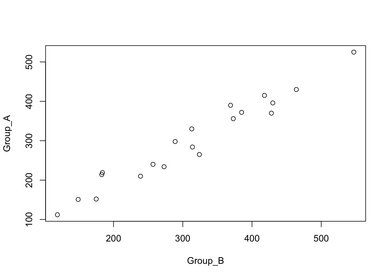
We take advantage of this pairing by comparing the two sales groups within each sales district and work with the differences. The differences in the data frame are formed as sales of group A minus sales of group B.
hist(Sales$Difference)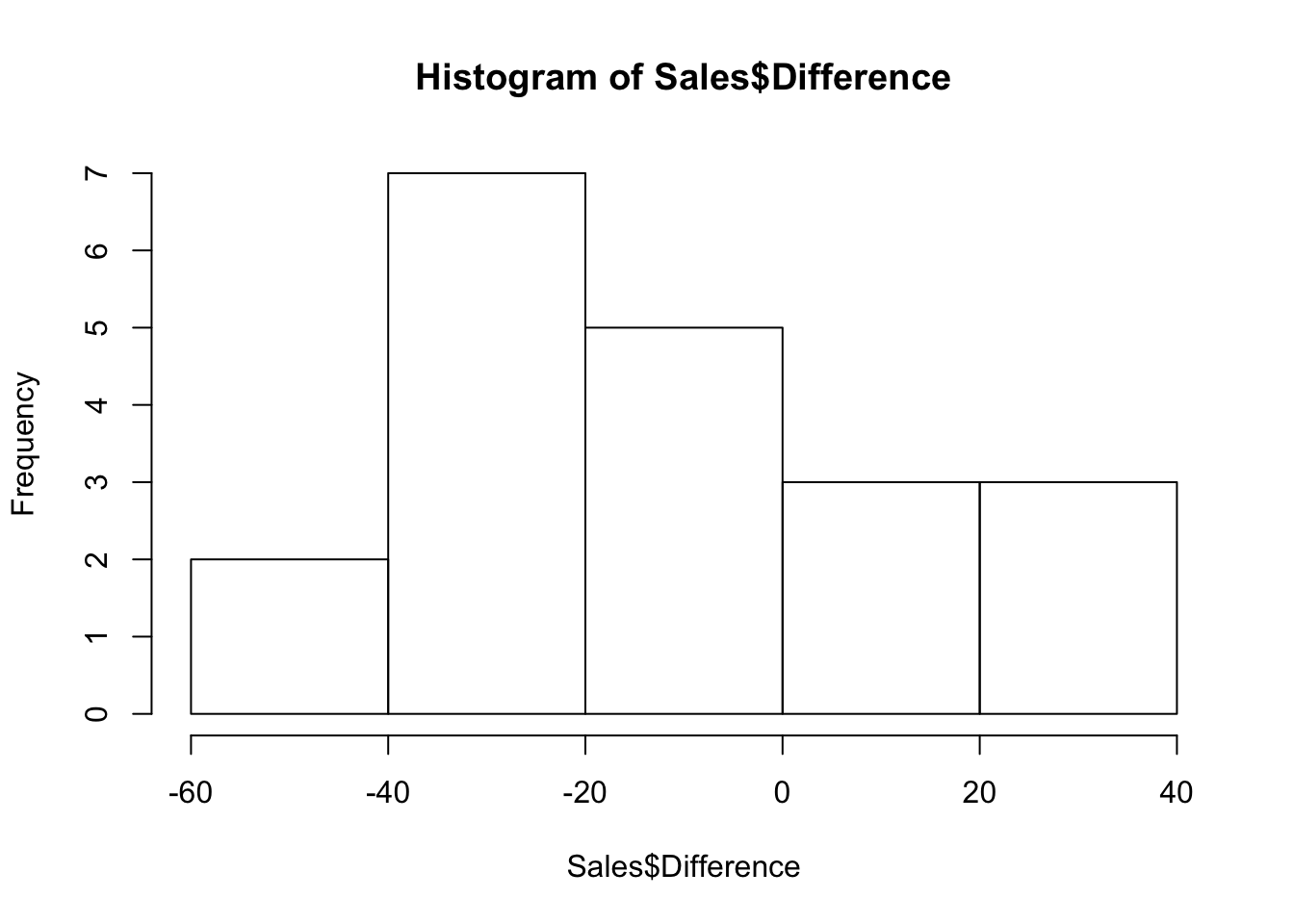
This is a small sample of districts, but the kurtosis is small and we have enough to meet the sample size condition.
require(moments)
kurtosis(Sales$Difference)-3
## [1] -0.7059701All we have left is to compute the needed statistics and either form a one-sample test or confidence interval for the average of the differences.
n <- length(Sales$Difference)

xbar <- mean(Sales$Difference)
s    <- sd(Sales$Difference)

t_quant <-qt(0.025, df=n-1)
The confidence intervals for \(\mu_A - \mu_B\) is
ci <- xbar + c(-t_quant,t_quant) * s/sqrt(n)
ci
## [1] -0.9818521 -26.0181479Since both endpoints are negative, we conclude \(\mu_B\) is statistically significantly larger.