18 Inference for Counts
The methods in this chapter resemble those in Chapter 5, with the addition of the p-value for the chi-squared statistic that appears in the summary of a contingency table using the CrossTable from the package gmodels. We also use some special functions for manipulating numbers as characters. The main functions illustrated in this chapter are
mosaicplotdraws mosaic plotsCrossTableoptionally shows the chi-squared statistic for a contingency tablepasteconverts a number into a character stringsubstrselects a subset of the characters in a stringtablegenerates a frequency distributionpchisqcomputes the tail probability of a chi-squared distributiondpoiscomputes Poisson probabilities
18.1 Analytics in R: Retail Credit
Begin the exercise by reading the data into a data frame.
Retail <- read.csv("Data/18_4m_retail.csv")
dim(Retail)
## [1] 630 3Each row of these data describes the current status and source channel (how the customer came to sign up for credit) of a customer of this retailer.
head(Retail)## Customer Status Channel
## 1 1000035 Current Web site
## 2 1008640 Current In store
## 3 1036244 Closed In store
## 4 1045205 Current Mailing
## 5 1049389 Late payment In store
## 6 1058492 Current Web siteHere’s the mosaic plot. The formula syntax of mosaicplot resembles that used with plot and lm, but it requires you to put the response on the right-hand side of the ~ to have it appear on the y-axis. The coloring here helps highlight the dependence. The colored “slices” would have equal height in the absence of dependence, producing a layered cake appearance with flat divisions.
mosaicplot(Channel ~ Status, data=Retail, col=c('orange','green','lightblue'))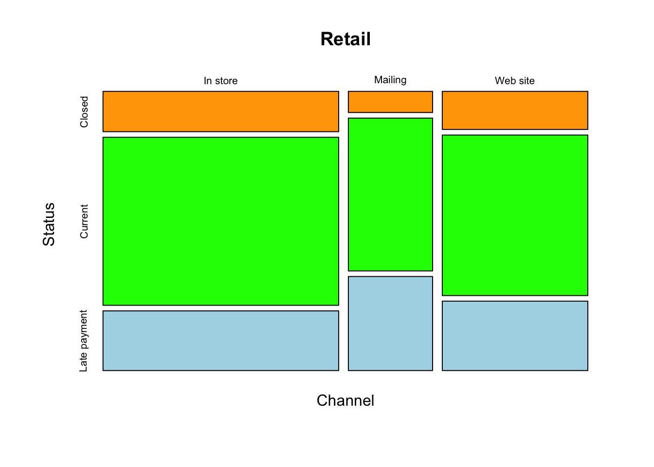
In the case of these data, the lack of a common horizontal split indicates the presence of dependence. In particular, customers originating in the mailing channel have a higher proportion of late payments and a lower proportion of closed accounts.
Next obtain the contingency table, with the chi-squared statistic added. The cells of the table show, by default, the contribution to the overall chi-squared statistic from the count in that cell. As suggested by the mosaic plot, the big contributions to \(\chi^2\) come from cells in the mailings column.
require(gmodels)
with(Retail,
     CrossTable(Status, Channel,
                chisq=TRUE,                               # add chi-squared
                prop.c=FALSE, prop.r=FALSE, prop.t=FALSE  # suppress these other contents
                ))
##
##
## Cell Contents
## |-------------------------|
## | N |
## | Chi-square contribution |
## |-------------------------|
##
##
## Total Observations in Table: 630
##
##
## | Channel
## Status | In store | Mailing | Web site | Row Total |
## -------------|-----------|-----------|-----------|-----------|
## Closed | 48 | 9 | 28 | 85 |
## | 0.572 | 2.647 | 0.076 | |
## -------------|-----------|-----------|-----------|-----------|
## Current | 200 | 65 | 118 | 383 |
## | 0.190 | 0.267 | 0.026 | |
## -------------|-----------|-----------|-----------|-----------|
## Late payment | 71 | 40 | 51 | 162 |
## | 1.483 | 3.895 | 0.002 | |
## -------------|-----------|-----------|-----------|-----------|
## Column Total | 319 | 114 | 197 | 630 |
## -------------|-----------|-----------|-----------|-----------|
##
##
## Statistics for All Table Factors
##
##
## Pearson's Chi-squared test
## ------------------------------------------------------------
## Chi^2 = 9.158316 d.f. = 4 p = 0.05726189
##
##
## 18.2 Analytics in R: Detecting Accounting Fraud
Again, build a data frame from the file.
Fraud <- read.csv("Data/18_4m_fraud.csv")
dim(Fraud)
## [1] 135 2These 135 invoices identify ID numbers and the dollar amounts.
head(Fraud)## Invoice Amount
## 1 6562307 54030.55
## 2 5546585 11692.67
## 3 6864692 45567.71
## 4 8454759 1343.58
## 5 4712204 24120.22
## 6 1834270 6922.19For this exercise, we need the first digit of each amount. To get that digit, start by converting these amounts into character strings using the function paste.
str <- paste(Fraud$Amount)
str[1:3]                     # the first 3 strings
## [1] "54030.55" "11692.67" "45567.71"The function substr (substring) extracts a portion of a string. For example, to get the characters in the third through fifth position:
substr("ABCDEF", 3, 5)## [1] "CDE"We want the first character of each digit string.
substr("123",1,1)## [1] "1"substr expands to a vector, so we can convert to string all of the amounts in this column of the data frame at once.
digit <- substr(Fraud$Amount,1,1)
digit[1:3]
## [1] "5" "1" "4"Next use table to get counts of these digits and save the results in a vector named obs, short for “observed counts”.
obs <- table(digit)
obs
## digit
## 1 2 3 4 5 6 7 8 9
## 26 31 22 18 13 10 11 2 2The chi-squared statistic compares these observed counts to the expected number based on Benford’s Law. We can use R to compute the expected counts. (See the textbook for the formula for Benford’s Law in the appendix of Chapter 18.)
n <- length(digit)

expect <- n * log10(1 + 1/(1:9))  # base 10 log
expect[1:3]
## [1] 40.63905 23.77232 16.86673The chi-squared statistic is then
chisq <- sum( (obs-expect)^2/expect )
chisq
## [1] 19.07708The p-value is the upper tail beyond this value of the chi-squared distribution with 9-1=8 degrees of freedom.
1 - pchisq(chisq, df=8)## [1] 0.014452818.3 Analytics in R: Web Hits
Read the data into a data frame.
Hits <- read.csv("Data/18_4m_web_hits.csv")
dim(Hits)
## [1] 685 2Each row gives a user identifier and the number of clicks on ads during a session by each user.
head(Hits)## UserID Clicks
## 1 7674 0
## 2 13568 1
## 3 14430 0
## 4 30416 0
## 5 36437 0
## 6 40732 1Use table to get the counts for how many users click on 0, 1, 2, … ads.
counts <- table(Hits$Clicks)
counts
##
## 0 1 2 3 4 5
## 368 233 69 13 1 1The counts for 4 or more are too small for the chi-squared statistic, so combine these with those for 3 clicks, which in spite of its label now represents “3 or more” clicks.
counts <- counts[1:4]
counts[4] <- counts[4]+2
counts
##
## 0 1 2 3
## 368 233 69 15To get the corresponding Poisson expected counts, we need the average number of clicks (identified as \(\lambda\) in the textbook).
lam <- mean(Hits$Clicks)
lam
## [1] 0.6116788The expected counts are then (be careful with the last probability; it is for 3 or more, not just 3). The calculation involving ppois computes \(P(X \ge 3) = 1 - P(X \le 2)\) for a r.v. \(X\) that has a Poisson distribution with parameter lam (\(\lambda\)).
n <- sum(counts)
expect <- n * c( dpois(0:2,lambda=lam), 1-ppois(2, lambda=lam) )
expect
## [1] 371.57102 227.28213 69.51183 16.63503The rest of the calculation proceeds as in the prior example.
chisq <- sum( (counts - expect)^2/expect )
chisq
## [1] 0.3426401The p-value is much too large to reject \(H_0\).
pval <- 1 - pchisq(chisq, 2)
pval
## [1] 0.8425519