16 Statistical Tests

As in the prior chapter on confidence intervals, we use R as a powerful calculator to illustrate the calculations. The hard part in these examples lies not in the calculations but in determining the appropriate hypotheses. The main functions emphasized here are:

• pnorm computes the p-value from the z-statistic
• pt finds the p-value for a t-statistic

16.1 Analytics in R: Do Enough Households Watch

This case concerns proportions, so we do not have to read the data from a file. Our first task is to label the relevant statistics given in the problem.

n    <- 2500
phat <- 0.06
 
p_0  <- 0.045    # hypothesized proportion

z <- (phat - p_0)/sqrt(p_0 * (1-p_0)/n)
z

## [1] 3.617873

Now use pnorm to find the p-value, the area under the normal curve outside (to the right of) \(z\). Because pnorm returns the area to the left of \(z\) (i.e., pnorm(z) = \(P(Z \le z)\)), the p-value needed in this example is 1 minus the value returned by pnorm.

1 - pnorm(z)

## [1] 0.000148517

16.2 Analytics in R: Comparing Returns on Investments

First read the data that gives the returns on IBM stock.

IBM <- read.csv("Data/16_4m_ibm.csv")
dim(IBM)

## [1] 72  2

These are monthly returns over 6 years.

head(IBM)

##      Date    Return
## 1 1/29/10 -0.065011
## 2 2/26/10  0.043468
## 3 3/31/10  0.008572
## 4 4/30/10  0.005848
## 5 5/28/10 -0.023953
## 6 6/30/10 -0.014210

R does not automatically read the dates as dates; it reads them as character strings and builds a factor. For plots, we need to convert these strings into dates. We use the lubridate package for that. (See Chapter 2 for more examples of dates.)

require(lubridate)    # require loads the package only if it is not already present
dates <- mdy(IBM$Date)

Now we can plot the returns with a reasonable date axis.

plot(dates, IBM$Return, type='l')
abline(h=0, col='gray')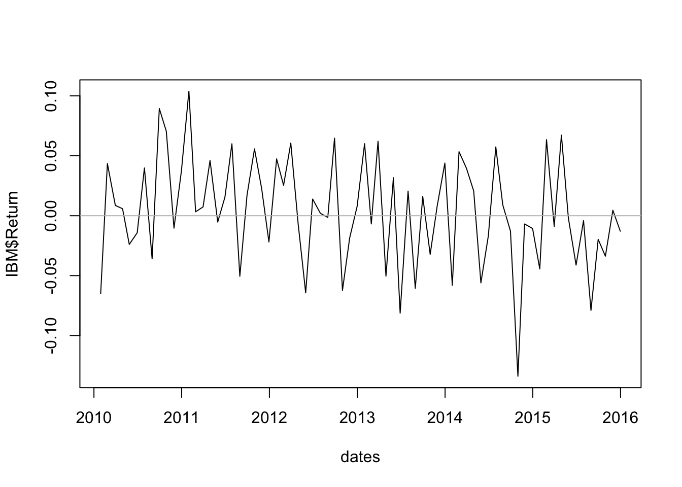

There doesn’t seem to be a time trend, so collapse the series (ignore the time variable) and inspect the histogram of returns.

hist(IBM$Return)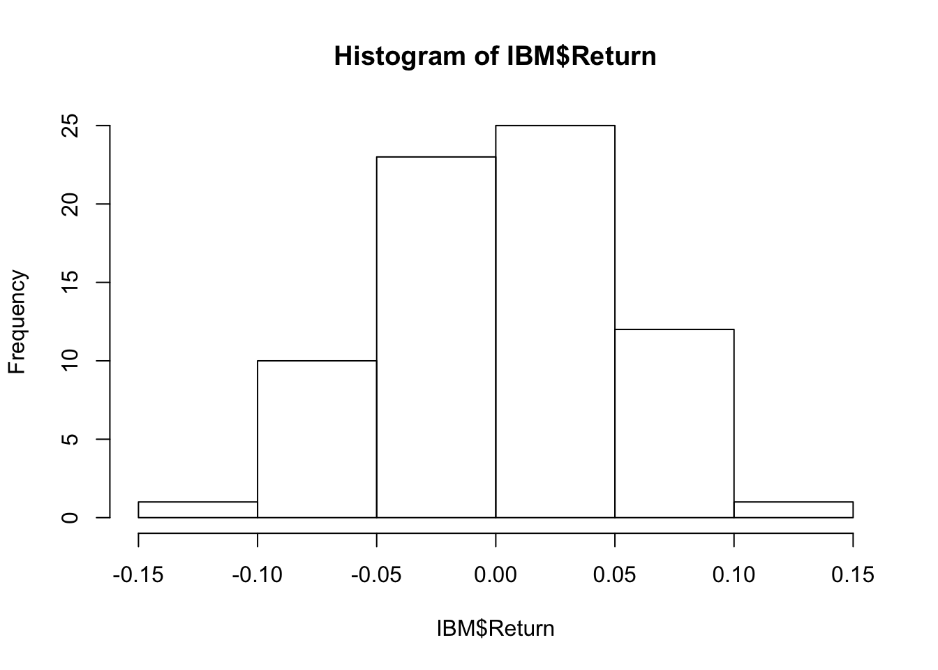

The distribution is reasonably symmetric, so we probably satisfy the sample size condition. The excess kurtosis is very small.

require(moments)

kurtosis(IBM$Return)-3

## [1] 0.06170312

Now define the relevant sample characteristics and use these to find the t-statistic. When done in this style, your expression for the t-statistic looks just like the formula in the text.

n    <- length(dates)
xbar <- mean(IBM$Return)
s    <- sd(IBM$Return)

mu_0 <- 0.0015

t <- (xbar-mu_0)/(s/sqrt(n))
t

## [1] 0.374721

The function pt computes the p-value, which indicates that the test is not statistically significant.

1 - pt(t, df=n-1)

## [1] 0.3544925