9 Random Variables

As in the prior two chapters, there’s nothing in this chapter than requires R for calculations. The only point worth making that might be of some interest is that R does make it easy to draw samples from various probability distributions. For example, suppose we have a random variable with the following probability distribution.

x   <- 1:10                                          # possible values x

p_x <- c(0.2, 0, 0.3, 0.1, 0, 0, 0, 0.35, 0, 0.05)     # probabilities P(X = x) = p(x)

By setting the optional type argument of plot to be “h”, we can get the plot function to draw vertical lines rather than just show points for the probabilities. By then calling the function points, we can add “balloons” to the tether lines to mark the probabilities. The bty argument removes the frame of the boundary box on the top and right side of the figure to give a more open look suitable for drawing a probability distribution.

plot(x,p_x, type='h', col='gray', ylab="p(x)", bty='l')  # bty controls the boundary box, see par
points(x,p_x, pch=19)                                    # pch=19 generates a solid ball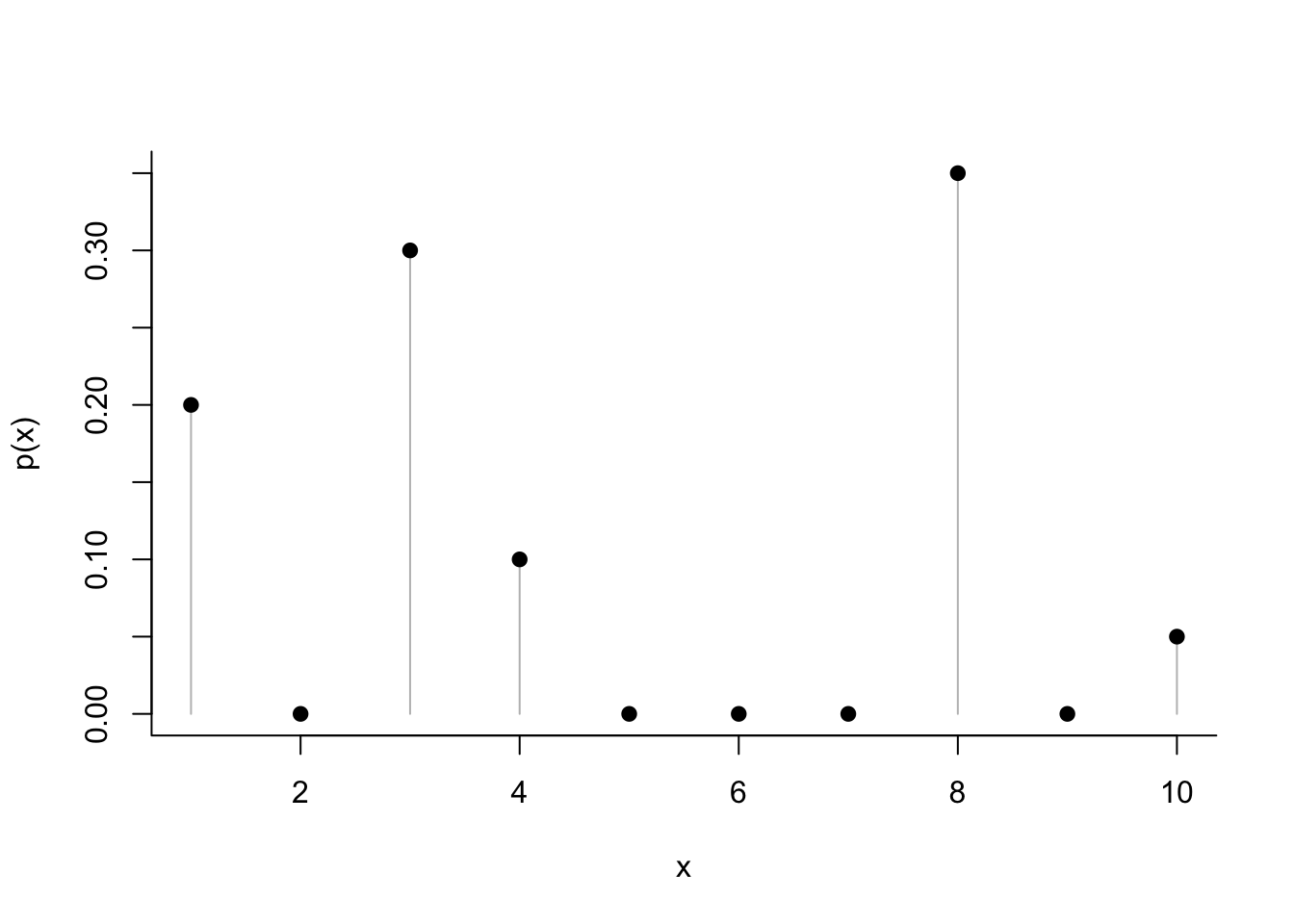

R can easily verify that the values meet the conditions for a probability distribution: all are positive and the sum is 1.

sum(p_x) == 1

## [1] TRUE

all(0 <= p_x)

## [1] TRUE