1 Introduction
This on-line supplement offers “Analytics in R” examples that show how to reproduce the statistical results and various plots that appear in the textbook Statistics for Business by Robert Stine and Dean Foster. Most chapters of this book include examples of data analyses. The third edition add a section called “Analytics in Excel” to the text. These notes show these same examples done with R. The coverage here is not a replacement for the text. These notes presume you’re also reading along in the book, and so offer only limited discussion of the goals of each analysis. The focus in the presentation here is how to get the results. You need to read in the textbook for a complete discussion of the motivation and ultimate message.
The first chapter does not have an analytics example, so this is a good place to mention some things about R itself. Keep in mind that just as our textbook provides tips on using Minitab, JMP, and Excel for statistics, these notes can only begin to show the capabilities of R. To keep this companion self-contained, this chapter has a few introductory examples to get you started. You can find much further information about R in books and on line, such as the material hosted at https://www.r-project.org and deposited at the Comprehensive R Archive Network (CRAN).
1.1 Basic R commands and syntax
R provides a host of mathematics that you can write out almost as if you read it from a book. For example, to find the square root of the sum of several numbers:
sqrt(23 + 44.23 + 12.5)## [1] 8.929166Or to get the average of 5 values:
(12 + 55 + 37 + 82 + 15)/5## [1] 40.2Notice that the result of each command is shown in a separate box preceded by two hash symbols (##). The hash symbol # in R denotes a comment. You will see this symbol throughout this companion to explain something that might otherwise be tricky.
R’s appeal for analytics comes from its vast collection of built-in statistical functions, such as the function mean that computes averages. For this function to be useful, we have to collect together batches of values. In R, collections of numbers are most often held in an object called a vector. You build a vector using the function named c, short for concatenate. The function assign represented by the arrow <- stores the value in a named object, a variable. (Many functions in R have short names in the style of c. That originates from R’s ancestry. R is an open source version of the language S which grew up at Bell Labs, home of the Unix operating system. Unix loves short command names, and R adopted many of these.)
x <- c(12, 55, 37, 82, 15, 66)  # create a vector named 'x' with 6 elements
mean(x)                         # find the average of the vector
## [1] 44.5Typing the name of the vector xprints the values in the vector.
x## [1] 12 55 37 82 15 66The function length tells you how many elements are in the vector x.
length(x)## [1] 6Vectors can also be rearranged into a table with rows and columns known as a matrix.
mat <- matrix(x, nrow=3, ncol=2)
mat
## [,1] [,2]
## [1,] 12 82
## [2,] 55 15
## [3,] 37 66Two indices locate items in a matrix.
mat[3,2]## [1] 66Matrices in R are special vectors, just arranged differently. We can still treat a matrix as a vector, as in finding its length.
length(mat)## [1] 6Vectors and matrices in R are important for a variety of statistical calculations; regression analysis exploits these objects heavily. They also have a limitation in R: they have to be all numbers or all strings. You cannot mix the type of elements. That’s an important limitation because data does mix information of different types. For holding data, R uses a different, more flexible data structure known as a data frame. Those appear in Chapter 2.
There’s not much value in putting 5 numbers into a vector if all we want is to find their average. The advantage comes when we want to manipulate those numbers in other ways as well. Once we have them collected into a vector, we can do lots of other things with them without having to type them again, such as find the smallest or largest element.
min(x)## [1] 12max(x)## [1] 82Of course, we don’t need R for these calculations; x has only 5 values. These same commands work, however, for much larger vectors.
Vectors in R collect numbers, but vectors are limiting when it comes to statistics. Statistics is most interesting when used to discover associations between different characteristics of people, places, and things. How are sales at Amazon related to prices at Walmart? How are tweets related to credit ratings? How is weight related to blood pressure?
Answers to questions like these require that we organize data. A vector is a natural way to collect the weights of several people, for instance, but we need to keep these weights matched to the corresponding blood pressures. Doing that requires us to organize our data into an object that resembles a table or spreadsheet. Most often in R, we will collect data into objects known as data frames.
That’s the topic of Chapter 2.
1.2 Plots
Plots are easy to produce in R. A plot of the vector x of 5 elements is not very interesting because it is so small, but you can see how easy it is to get a plot.
plot(x) # be careful: R is case sensitive (X and x are not the same)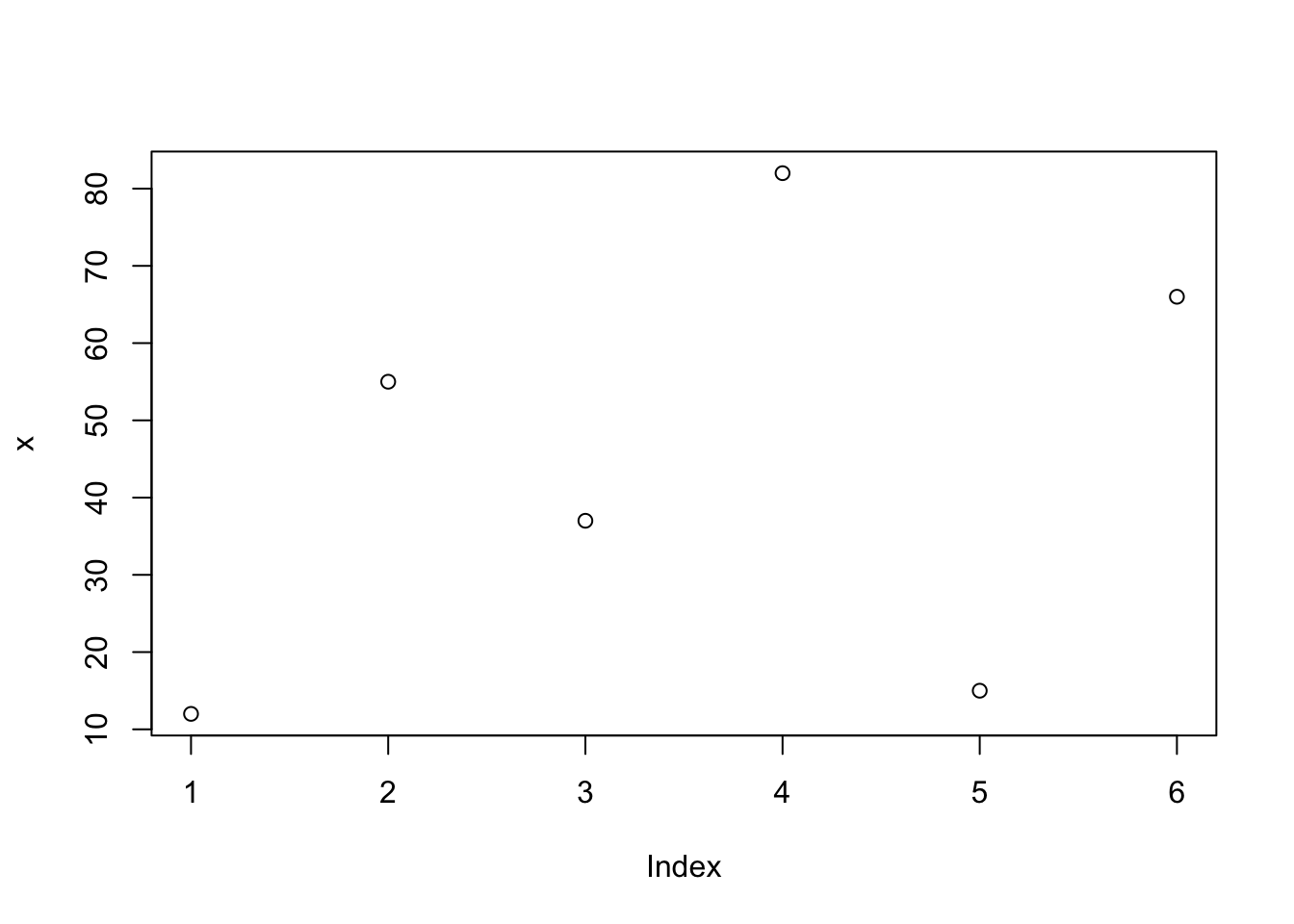
Figure 1.1: A plot of a vector with five values.
1.3 On the style of R in these chapters.
I have a few personal choices that appear often in these chapters, so I thought it would be worthwhile to mention them. They are totally personal choices, and others may use R differently.
Reading Data
I will use the standard R function read.csv to read data from a CSV file and return an R data frame. There are a number of notable alternatives to read.csv (such as read_csv from the so-called “Tidyverse” functions from Hadley Wickham), but read.csv is built into R. After I read a CSV file, I use the function dim to get the size of the resulting data frame and use head (or perhaps View) to see what the data look like. This being an introduction to statistics, the data files are very clean.
In these examples, I assume that you have loaded the data sets into a subdirectory named “Data” of the current working directory. You might need to read a bit more about R to learn how it manipulates files and directories on your computer. You can get a zip file with the data examples from my web page at http://www-stat.wharton.upenn.edu/~stine, located in the section on teaching and textbooks. Once you have this compressed archive, expand it on your system in a place that is easy to access from R. For example, on my system the current working directory has the source of these chapters.
getwd()## [1] "/Users/bob/books/AddisonWesley/one_semester/R/r_companion"I put all data files are in the “Data” subdirectory of this directory. You can also get the data files individually from my web site. Just replace the reference to the data subdirectory with the long URL shown in this example.
Data <- read.csv("http://www-stat.wharton.upenn.edu/~stine/R-companion/Data/02_bike_shop.csv")
Data
## Customer Club.Member Date Type Brand Size Amount
## 1 Oscar 0 52215 B Colnago 58 4625.00
## 2 Karen 1 6315 Tu Conti 27 4.50
## 3 Karen 1 61515 Ti Michelin 27 31.05
## 4 Bob 1 82115 B Kestrel 56 3810.00Strings
R allows both single and double quotes to delimit strings. The following two strings are the same.
s1 <- 'bob'
s2 <- "bob"
s1 == s2
## [1] TRUEMy personal convention is that I use double quotes for strings that I can choose freely, such as the title of a plot or label on a plot axis. For strings that have specific meaning within R, I use single quotes. For example, the string 'red' denotes the color red in R. I write this string with single quotes as a reminder that this specific string means something special in R.