6 Association between Numerical Variables
Association between numerical variables is analogous to association between categorical variables. There’s both a visual aspect (a scatterplot replaces the mosaic plot) and a numerical summary (correlation replaces Cramer’s V). The key functions in this chapter are
lmfinds the correlation lineplotdraws scatterplots of numerical data using model syntaxablineadds lines to scatterplotscorcomputes the correlation
In addition, we show examples of the visual test for association.
6.1 Analytics in R: Locating a new store
The data in this example describe sales in dollars of 55 stores and include the distance to the nearest competitor and the size of the store in square feet.
Location <- read.csv("Data/06_4m_location.csv")
dim(Location)
## [1] 55 3head(Location)## Sales Distance Sq.Ft
## 1 2461894 4.0 8340
## 2 3164163 9.0 10740
## 3 2759710 5.0 10070
## 4 1739977 1.5 5910
## 5 2143862 3.5 7210
## 6 1791770 2.0 6360The function lm (short for “linear model”) computes the correlation line (also known as the least-squares line). The “formula syntax” shown below for identifying the variables in the line is common in regression modeling in R. The name to the left of the ~ is the response and will be shown on the y-axis in plots. The variable to the right is the explanatory variable. This style of identifying the variables in a regression model uses the data argument to identify the data frame that holds the variables (rather than with).
lm(Sales~Distance, data=Location)##
## Call:
## lm(formula = Sales ~ Distance, data = Location)
##
## Coefficients:
## (Intercept) Distance
## 1762412 159305We can use the formula syntax to describe the variables for the scatterplot as well. Both plot and lm share this style of arguments.
plot(Sales ~ Distance, data=Location)

abline(lm(Sales~Distance, data=Location), col='red')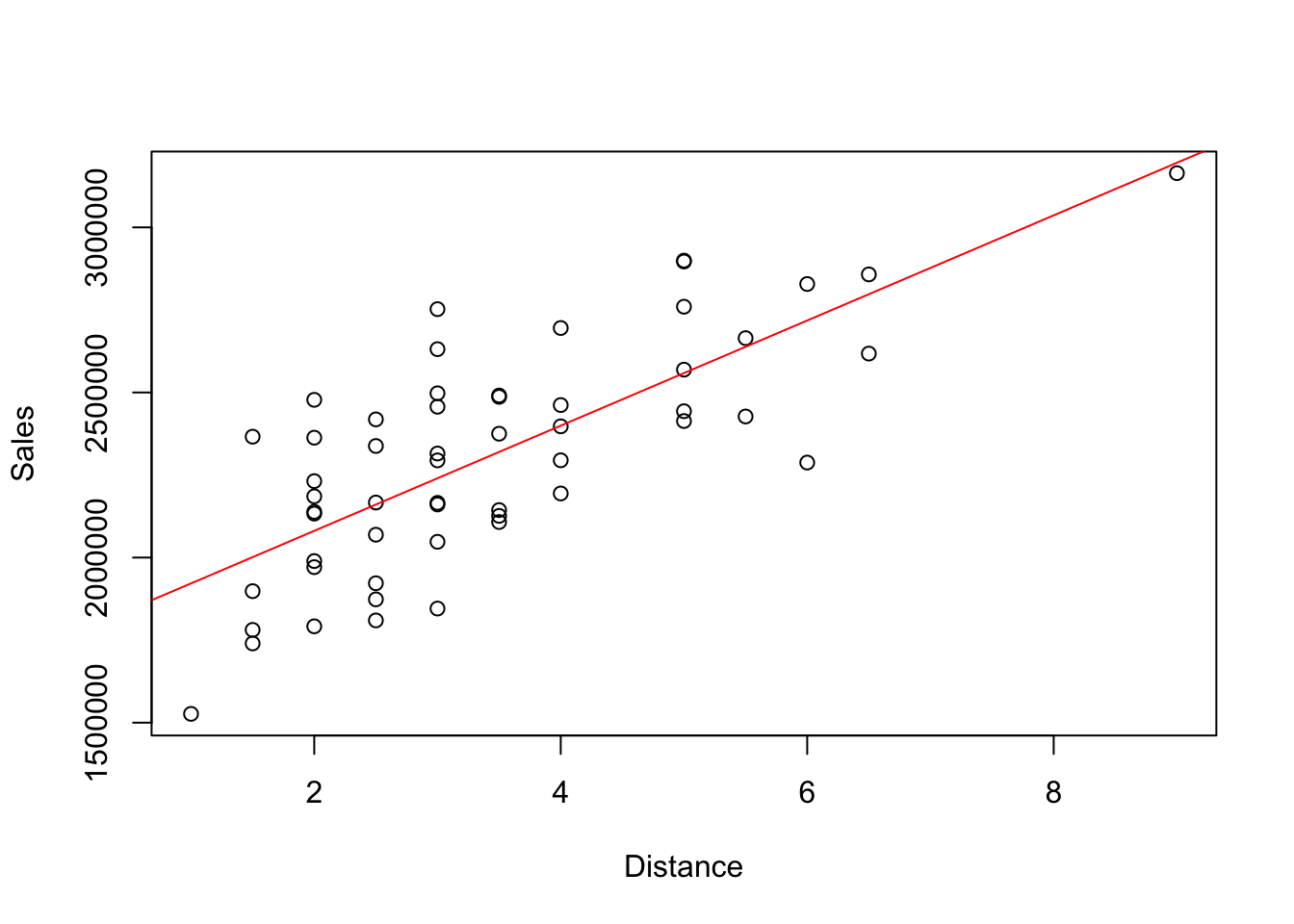
The function cor (with just one “r”) computes the correlation between a pair of variables.
with(Location,
     cor(Sales, Distance))
## [1] 0.7414622If given a data frame or matrix of numerical variables, cor returns the correlation matrix. In this example, we can find the correlation between sales and distance as seen above, as well as the correlation between these two variables and the number of square feet. For example, the correlation between sales and square feet is about 0.8557.
cor(Location)## Sales Distance Sq.Ft
## Sales 1.0000000 0.7414622 0.8557274
## Distance 0.7414622 1.0000000 0.8777983
## Sq.Ft 0.8557274 0.8777983 1.0000000Here’s an example of the visual test for association. This function is defined in the file “functions.R” which is available on line from the site where you obtained the data. The syntax of this function is just like that used by plot and lm. If you can easily pick out the plot of the original pair of variables as shown above from a collection of scrambled plots, then strong association is present. The harder you find it to pick out the original scatterplot, the weaker the association.
source("functions.R")
visual_test_for_association(Sales~Distance, data=Location)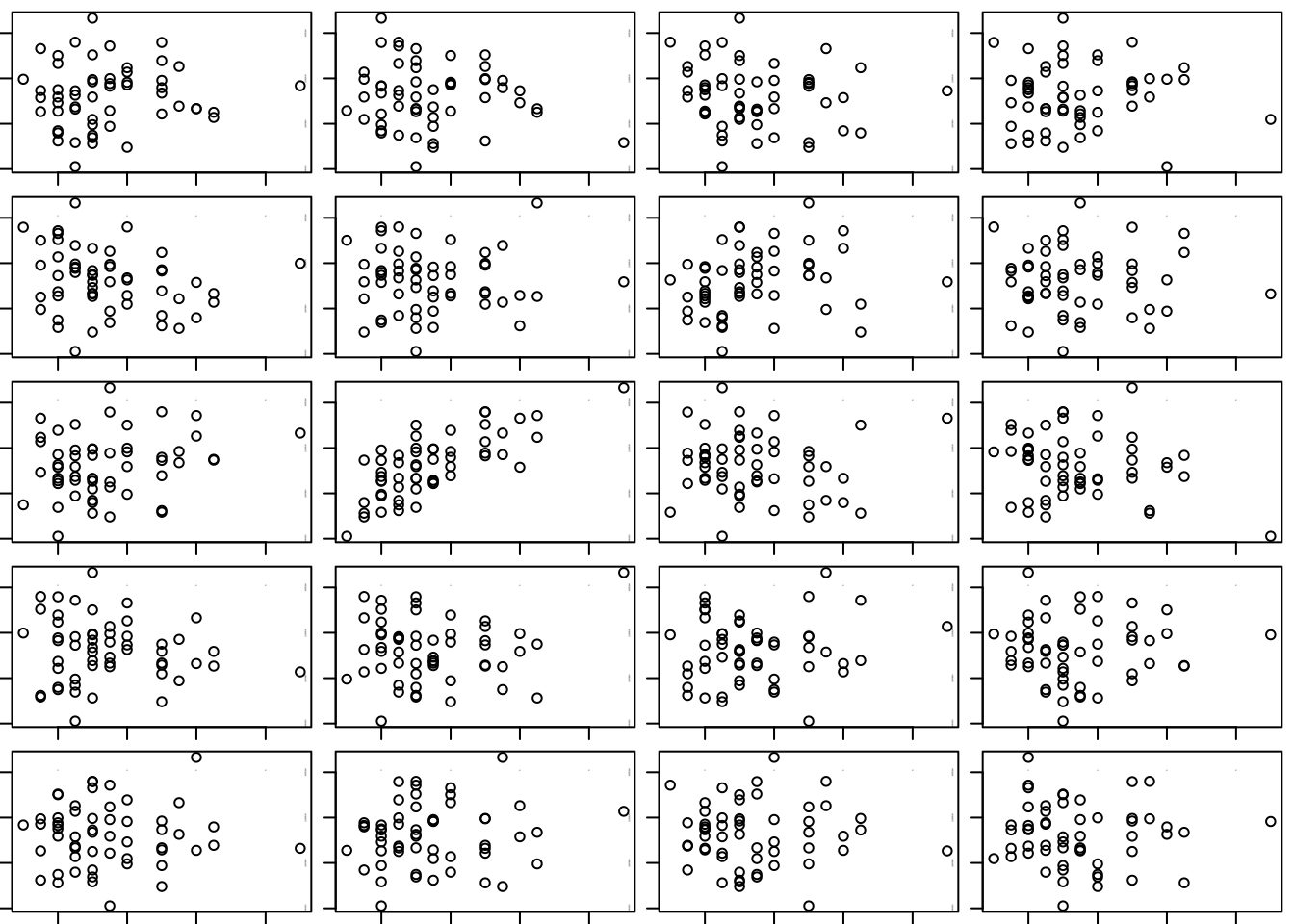
## [1] 3 2In this example, the original is the second plot in the third row. It’s not to hard to recognize, but does not jump off the page. We’d call that moderate association.